Research Article

Uncertainty Quantification of Sea Waves - An Improved Approach

Sayyed Mohsen Vazirizade¹, Achintya Haldar*¹ and J. Ramon Gaxiola-Camacho³

¹Department of Civil and Architectural Engineering and Mechanics, University of Arizona, USA

²Department of Civil Engineering, Autonomous University of Sinaloa, Mexico

Submission: April 23, 2019; Published: May 14, 2019

*Correspondence author: Achintya Haldar, Professor at the Department of Civil and Architectural Engineering and Mechanics, University of Arizona, Tucson, AZ, USA

How to cite this article:Sayyed Mohsen Vazirizade, Achintya Haldar, J Ramon Gaxiola-Camacho. Uncertainty Quantification of Sea Waves - An Improved Approach. Oceanogr Fish Open Access J. 2019; 9(5): 555775. DOI: 10.19080/OFOAJ.2019.09.555775

Abstract

Sea waves are important dynamic loadings for the design of offshore structures. Casual observations will indicate that the sea waves are very unpredictable and may not be modeled deterministically. To capture the unpredictable nature of the sea waves, they are generally expressed in terms of a joint probability density function of mean zero crossing period Tz and the significant wave height Hs. Estimation of parameters of the joint distribution can be very challenging, particularly considering the scarcity of data. The joint probability density function (PDF) of Tz and Hs is generally represented as the multiplication of a conditional distribution for Tz given Hs and the marginal distribution of Hs. The estimation of parameters of the joint PDF is addressed in this paper. The available information on North Atlantic, as reported by Det Norske Veritas (DNV), is considered to document its applicability. DNV reported values for all the required parameters. They are considered as the reference values. Using the Maximum Likelihood Method (MLM), the three parameters of the Weibull distribution for the marginal distribution of Hs are estimated. Assuming Hs can be represented by a two-parameter Weibull distribution, they are also estimated. To compare different alternatives, their Root-Mean-Square-Error values are also estimated. It can be observed that the proposed MLM to estimate the parameters of Hs is superior to that of proposed by DNV.

Keywords: Wave height; Weibull distribution; Wave modeling; Lognormal distribution; Scatter diagram

Introduction

Sea waves are one of the most important dynamic loadings for the design of offshore structures. The dynamic characteristics of sea waves, in terms of the wave height and frequency contents, are extremely important for the design. Casual observations will indicate that the sea waves are very unpredictable and may not be modeled deterministically. For the successful design of offshore structures, the sea wave loading needs to be mathematically represented as accurately as possible. The authors believe that the most efficient way to quantify the uncertainty in the sea wave loading is statistically. It will require the collection of sea state data at a particular site. And then try to fit a mathematical model to the data. Obviously, the precision of the prediction will increase with the size and types of the data collected and their accuracy. Since the mathematical model will represent the actual sea states, it is expected to be acceptable to the engineering community. At present, the reliability analyses of both onshore and offshore structures are expected from the engineering profession so that communities are not exposed to unacceptable risk [1-4].

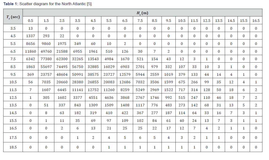
The sea wave data important to this study are the significant wave height Hs which is the average of the upper third of the wave heights and the mean of the zero up-crossing period Tz which is the average value of the time between successive up-crossing of the still water. The information on them is usually recorded in three-hour duration and both parameters are estimated for this duration. After collecting the data over a period, the information is summarized in a tabular form, generally known as the scatter diagram. Table 1 shows the scatter diagram for the North Atlantic [5]. It represents the total number of observations for each pair of Hs and Tz. The values of Hs and Tz shown in Table 1 are the center of each interval, i.e., when Hs is 1.5 m, it represents the interval of 1 and 2 m. Tz is defined similarly (Table 1).

Uncertainty Quantification - Methodology

With the availability of the data shown in Table 1, the major challenge is to find an appropriate mathematical model. A literature review will indicate the joint probability density function (PDF) of Tz and Hs is generally represented as the multiplication of a conditional distribution for Tz given Hs and the marginal distribution of Hs [6-10]. It can be mathematically represented as:

The joint distribution model represented by Eq. 1 is very helpful since it includes both frequency content and amplitude of the sea waves [11]. The most common distribution used for the conditional PDF (the first term on the right hand side of Eq. 1) is lognormal [12]. Weibull and Rayleigh distributions are generally used for the marginal distribution of Hs (the second term on the right hand side of Eq. 1) [13,14]. Subsequently, it was reported that lognormal distribution for conditional distribution Tz given Hs and Weibull for the marginal distribution of Hs are the best choices [15,16]. Even though this model was initially developed for the Norwegian Sea, it was shown that this model could be adjusted for any locations [17]. Finally, Det Norske Veritas (DNV) [18] proposed lognormal distribution for the conditional distribution and Weibull distribution for the marginal distribution of Hs and showed that these were the reliable mathematical models, and they are considered in this paper.

Conditional PDF - Lognormal Distribution

The conditional PDF of | ( | ) TZ HS Z S f t h considering it is lognormally distributed can be mathematically expressed as:

where TZ |HS λ and | TZ HS ζ are the two parameters of the lognormal distribution [19]. They are essentially mean and standard deviation of the natural logarithm of the original data. For the conditional lognormal distribution, the two parameters can be shown to be 2 Z | S 0 1 a T H s λ = a + a h and | 0 1 2 exp( ) TZ HS s ζ = b + b b h [20]. Based on the data in Table 1 for each interval of hs (each column in Table 1; there are 17 columns; in general it can be any other number), TZ |HS λ and TZ |HS ζ are estimated. Using 17 values of TZ |HS λ , the parameters a0, a1 and a2 are estimated by curve fitting the data. Similarly, b0, b1 and b2 are estimated using the 17 values for TZ |HS

Marginal Distribution of Hs - Weibull Distribution

>

The Weibull distribution is a type III extreme value distribution. As mentioned earlier, Weibull distribution is considered for Hs in this study. The PDF and cumulative distribution function (CDF) of , ( ) s hS s H f h can be expressed as:

where α ,β ,γ are the shape (slope), scale and location (shift or threshold) parameters. α ,β are always positive. When β =1, Eq. 3 will represent the Exponential distribution, and when β = 2 , it will represent the Rayleigh distribution. However, γ can be positive or negative. If it is zero, the three-parameter Weibull distribution will reduce to two-parameter Weibull distribution. γ is the minimum value for which the CDF is non-zero. According to the definition of Hs which is the average of the upper third of the wave heights, it is always positive and cannot be zero. Furthermore, there some observations for the first interval of Hs, for example, in Table 1, 13 observations exist for the range between zero and one. Consequently, the maximum acceptable value for γ is the upper range of the first interval, i.e., 1 for Table 1.

Maximum Likelihood Estimation

In this study, the estimation of parameters of the Weibull distribution is studied considering the type of information given in Table 1. There are several methods available to estimate the parameters of a distribution. However, estimation of the three parameters of Weibull distribution can be challenging. The level of difficulty increases significantly when the available data are grouped as shown in Table 1. The Maximum Likelihood Method (MLM) is considered to estimate the three parameters of Weibull distribution [20]. The basic concept of MLM is that if there are n observations of a random variable, then the estimated value of the parameter is the most likely to produce these values. The underlying mathematical concept can be developed in the following way. Suppose, X is a random variable with parameter which needs to be estimated with n data. Denoting the PDF of X as ( , ) Xfxθ and assuming the likelihood of observing xi’s is proportional to their corresponding PDF, the likelihood function can be defined as:

The data in Table 1 are grouped in k intervals, i.e. 0 1 1 2 1 [ , ],[ , ], , [ , ] k k t t − t t − t t − − … . The probability of an observation falling in the jth interval is:

where F(t,θ ) is CDF of t for a given value of θ. Hence, the likelihood function of the Weibull parameters for a grouped sample can be expressed as:

where k is the total number of the groups, nj is the frequency or the number of observations for the jth group, and 1 k j j n n = Σ = . The three parameters of the Weibull distribution are α, β and γ and they need to be estimated by the available data using MLM. Equation 7 can be re-written as:

Since working with summation is easier than multiplication and taking logarithm from both sides does not change the location of the maximum values, which is of interest, the natural logarithm of Eq. 8 can be shown to be:

By taking the derivative of Eq. 9 with respect to α,β and γ, respectively, one by one, the maximum likelihood estimation of three parameters can be obtained. This operation will result in the following three equations:

The data shown Table 1 are used to calculate the mean (𝜇) and standard deviation (𝜎) of the whole sample. Weibull parameters are estimated using MLM using Eq. 10. Assuming, the distribution of Hs can be described by two-parameter Weibull distribution, they are also estimated. The information is summarized in Table 2. The Weibull parameters estimated by DNV for the data shown Table 1 are available [5]. The information is summarized in Table 2. To compare different alternatives, the Root-Mean-Squared- Error (RMSE) of each model is calculated with respect to the data in Table 1. They are summarized in the last column in Table 2.

Several important observations can be made from the information summarized in Table 2. The estimated RMSE values clearly indicate that the proposed MLM-based parameter estimation for Hs using the three parameters Weibull distribution is superior to that of the method used by DNV, at least for the data for the North Atlantic region. The results also indicate that the very commonly used two-parameter Weibull distribution to model the marginal distribution of Hs is not as accurate as the three-parameter Weibull distribution. Six parameters of the conditional lognormal distribution are estimated next (Table 3). The information is summarized in three ways in Table 3. The values reported by DNV are summarized in the first row. They used ao = 0.7. Assuming ao = 0.7, the remaining 5 parameters are estimated, and the information is summarized in row 2 of Table 3. Without assuming a fixed of 0.7 for ao, all 6 parameters are estimated for the data given in Table 1. The information is summarized in the third row in Table 3 (Table 3).

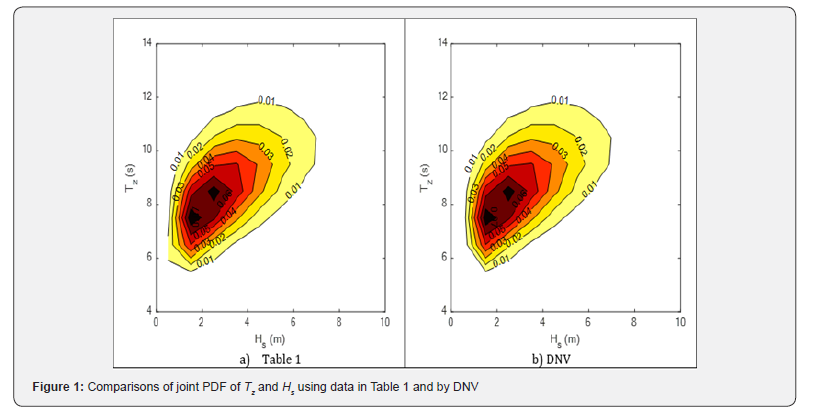
To study the implications of different values of the parameters to define the joint PDF of Tz and Hs, they are plotted for different cases. The joint PDFs of the data given in Table 1 and parameters suggested by DNV are plotted in Figures 1a & 1b, respectively. They are essentially the same except at the region close to the origin (Figure 1). The same information is plotted in Figure 2 using the parameters proposed in the paper. Figures 2a & 2b are essentially the same. Figures 2c & 2d clearly indicate the deficiencies in using the two-parameter Weibull distribution for Hs as documented in Table 2. The authors recommend the MLM-based parameters estimation procedure demonstrated in this paper to quantify uncertainty in the sea waves (Figure 2).

Conclusion

To capture the unpredictable nature of the sea waves, they are generally expressed in terms of a joint PDF of Tz and Hs. Estimation of parameters of the joint distribution can be very challenging, particularly considering the scarcity of data when Tz and Hs approach zero. The available information on North Atlantic, as reported by DNV, is considered in this study. DNV reported values for all the required parameters. They are considered as the reference values in this study. Using the MLM, the three parameters of the Weibull distribution for Hs are estimated. Assuming Hs can be represented by two-parameter Weibull distribution, they are also estimated using MLM. To compare different alternatives, their RMSE values are also estimated. It can be observed that the proposed MLM to estimate the parameters of Hs is superior to that of the method used by DNV. For the conditional lognormal distribution of Tz given Hs, assuming a specific value for a0 or a data-based value may not be critical, particularly for the North Atlantic region. The authors recommend the MLM-based parameters estimation procedure demonstrated in this paper to quantify uncertainty in the sea waves.

References

1. J R Gaxiola-Camacho, A Haldar, H Azizsoltani, F Valenzuela-Beltran, A Reyes-Salazar (2018) Performance-Based Seismic Design of Steel Buildings Using Rigidities of Connections. ASCE-ASME J Risk Uncertain Eng Syst Part A Civ Eng 4(1): 4017036.
2. H Azizsoltani, J R Gaxiola-Camacho, A Haldar (2018) Site-specific seismic design of damage tolerant structural systems using a novel concept. Bulletin of Earthquake Engineering 16(9): 3819-3843.
3. J R Gaxiola-Camacho, A Haldar, A Reyes-Salazar, F Valenzuela-Beltran, G E Vazquez-Becerra, et al. (2018) Alternative reliability-based methodology for evaluation of structures excited by earthquakes. Earthquakes and Structures 14(4): 361-377.
4. H Azizsoltani, A Haldar (2018) Reliability Analysis of Lead-Free Solders in Electronic Packaging Using a Novel Surrogate Model and Kriging Concept. J Electron Packag 140(4): 41003-41011.
5. D N Veritas (2010) DNV Environmental conditions and environmental loads. Recommended practice DNV-RP-C205.
6. O G Houmb and T Overvik (1976) Parameterization of wave spectra and long-term joint distribution of wave height and period. The first Insternational Conference on the Behaviour of Offshore Structures (BOSS-76) 144.
7. S Haver and S R Winterstein (2009) Environmental contour lines: A method for estimating long term extremes by a short-term analysis. Trans Soc Nav Archit Mar Eng 116: 116-127.
8. K J Eik and E Nygaard (2003) Statfjord Late Life Metocean Design Basis.
9. E M Bitner-Gregersen (2015) Joint met-ocean description for design and operations of marine structures. Appl Ocean Res 51: 279-292.
10. E M Bitner-Gregersen (2010) Uncertainties of Joint Long-Term Probabilistic Modelling of Wind Sea and Swell, 29th International Conference on Ocean, Offshore and Arctic Engineering.
11. E M Bitner-Gregersen and S Haver (1991) Joint Environmental Model for Reliability Calculations. The First International Offshore and Polar Engineering Conference. International Society of Offshore and Polar Engineers, United Kingdom.
12. S Haver (1985) Wave climate off northern Norway. Appl. Ocean Res 7(2) 85-92.
13. Nordenstrom (1973) A method to predict long-term distributions of waves and wave-induced motions and loads on ships and other floating structures. Chalmers University of Technology.
14. A Shariff and M H Hafezi (2012) Modelling significant wave height data of North Sea: rayleigh vs weibull distribution. Applied Mechanics and Materials 157: 652-657.
15. E M Bitner-Gregersen, A S Veritas, and S Haver (1989) Joint Long-Term Description of Environmental Parameters for Structural Response Calculation. 2nd international workshop on wave hindcasting and forecasting 21-32.
16. J Mathisen and E M Bitner-Gregersen (1990) Joint distributions for significant wave height and wave zero-up-crossing period. Appl Ocean Res 12(2): 93-103.
17. E M Bitner-Gregersen, E.H Cramer, and R Løseth (1995) Uncertainties of load characteristics and fatigue damage of ship structures. Marine Structures 8(2): 97-117.
18. G Sigurdsson and E Cramer (2000) Guideline for Offshore Structural Reliability Analysis-Examples for Jacket Platforms.
19. Haldar and S Mahadevan (2000) Probability, Reliability and Statistical Methods in Engineering Design, John Wiley.
20. G Sigurdsson, E Cramer, I Lotsberg, B Berge (1996) Guideline for Offshore Structural Reliability Analysis: Application to Jacket Platforms.