The Zero Truncated Poisson Burr X Inverse Exponential Distribution for Modeling Fracture Toughness and Taxes Revenue Data
Jehan A. Almamy1, Saeed Al-mualim1,2, M. S. Hamed1,3 and Haitham M. Yousof3
1 Management Information System Department, Taibah University, Saudi Arabia
2Department of Statistics, Sana’a University, Yemen
3 Department of Statistics, Mathematics and Insurance, Benha University, Egypt
Submission: September 27, 2018; Published: November 14, 2018
*Corresponding author: Haitham M. Yousof, Department of Statistics, Mathematics and Insurance, Benha University, Egypt.
How to cite this article: Jehan A. A, Saeed Al-mualim, M S Hamed, Haitham M Y. The Zero Truncated Poisson Burr X Inverse Exponential Distribution for Modeling Fracture Toughness and Taxes Revenue Data. Biostat Biometrics Open Acc J. 2018; 8(4): 555742. DOI: 10.19080/BBOAJ.2018.08.555742
Abstract
In this work, we derive a new inverse exponential continuous model via the zero truncated Poisson distribution with a strong physical interpretation. A round of mathematical properties are derived. The maximum likelihood method is considered for estimating the unknown parameter of our model. The new model is much better other important competitive models.
Keywords: Zero Truncated Poisson; Inverse Exponential; Maximum Likelihood; Modeling Real Data
Abbrevations: IE: Inverse Exponential; PDF: Probability Density Function; CDF: Cumulative Distribution Function; BXII: Burr XII; LxIE: Lomax IE; LLIE: Log-logistic IE; ZTP: Zero Truncated Poisson; PMF: Probability Mass Function; HRF: Hazard Rate Function; AIC: Akaike Information Criterion; HQIC: Hannan-Quinn Information Criterion; CAIC: Consistent Akaike Information Criterion; BIC: Bayesian Information Criterion; QF: Quantile Function
Introduction and physical motivation
The Inverse Exponential (IE) distribution was originally introduced by Keller & Kamath [1] and it has been derived and considered as a lifetime model. If a random variable (r.v.) X has an E distribution, the variable Y=x-1 will have an IE distribution. The probability density function (PDF) and cumulative distribution function (CDF) of the inverse exponential (IE) distribution are given by (for x≥0)

respectively, where 0a> is the scale parameter. In this paper we propose and study a new extension of the IE distribution using the zero truncated Poisson (ZTP) distribution. Suppose that a system has N subsystems which functioning independently at a given time where N has ZTP distribution with parameter .α It is the conditional probability distribution of a Poisson-distributed r.v., given that the value of the r.v. is not zero ()0.≠The probability mass function (PMF) of N is given by

Note that for ZTP r.v., the expected value (EN|α) and variance Var(N|α) are, respectively, given by

and

Suppose that the failure time of each subsystem has the Burr X IE  for short) defined by the CDF and PDF given by
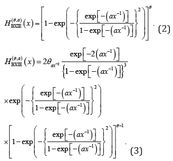
respectively, where a>0 is a scale parameter and 0θ> is the shape parameters.Let Yi denote the failure time of the ith subsystem and let  .Then the conditional CDF of X given N is

Therefore, the unconditional CDF of the PBXIE density function, as described in Ramos et al. (2015), can be expressed as
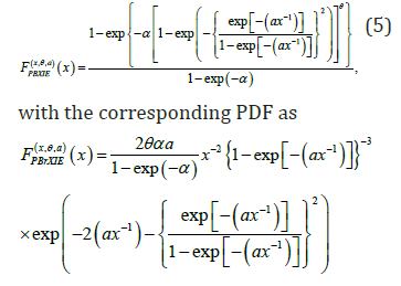
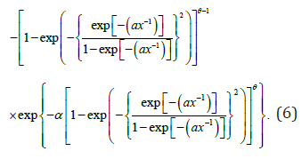
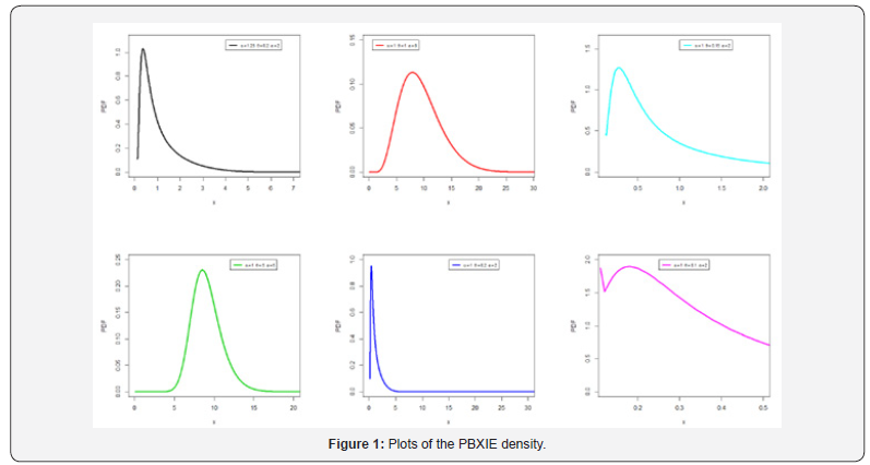
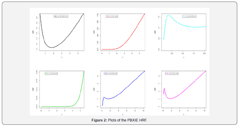
The hazard rate function (HRF) can be easily obtained via  Figure 1 shows that the PDF of the PBXIE model exhibits various shapes like right skewed symmetric and from Figure 2 we see that the HRF of the PBXIE model exhibits increasing, unimodal then bathtub and bathtub and unimodal then increasing hazard rates.
This paper is organized as follows
In Section 2, we derived some properties of the PBXIE model. Maximum likelihood (ML) method for the PBXIE model parameters under the uncensored case is addressed in Section 3. In Sections 4 potentiality of the PBXIE model is illustrated by means of two real data sets. Finally, Section 5 provides some concluding remarks.
Mathematical Properties
Useful expansions
Using the power series

the PDF in (6) can be written as

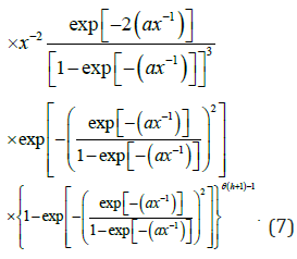
If |s|< 1 and c>0 is a real non-integer, the following power series holds

Applying (8) to (7) we have
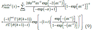
Applying the power series to the term  Equation (9) becomes
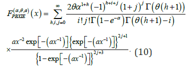
Consider the series expansion

Applying the expansion in (11) to (10) for the term  ,Equation (10) becomes


This can be written as

where

and  is the IE density with scale parameter
  Similarly, the CDF of the PBXIE model can also be expressed as

Where  is the IE density with scale parameter
Quantile and random number generation
The quantile function (QF) of ,X where  ,is obtained by inverting (5) as

Simulating the PBXIE r.v. is straightforward. If U is a uniform variate on the unit interval (0, 1); then the r.v. X=Q(U) follows (6).
Moments
The r(th) ordinary moment of ,X say follows from (12) as

Where
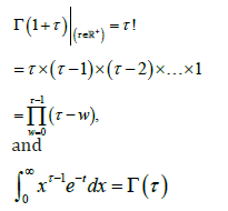
is the complete gamma function.
Incomplete moments
The r(th) incomplete moment of X is defined by

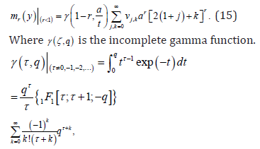
and []11,,F⋅⋅⋅ is a confluent hypergeometric function.
Generating functions
The moment generating function (mgf) of ,X say 

Moment of residual life
The ()thn moment of the residual life, say

uniquely determines ().FxThe ()thn moment of the residual life of Xis given by
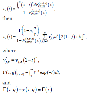
The mean residual life function or the life expectation at age t defined by

The MRL of X can be derived by setting 
Moment of reversed residual life
The ()thn moment of the reversed residual life, say
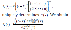
Then, the ()thn moment of the reversed residual life of X comes from
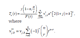
The mean inactivity time (the mean reversed residual life function) is given by

The mean inactivity time of the new is obtained easily by setting n=1 in Tn(t)
Estimation
Useful expansions
In this work we will consider the ML Method for estimating the unknown parameter of our model. The log likelihood ()logL can be expressed as
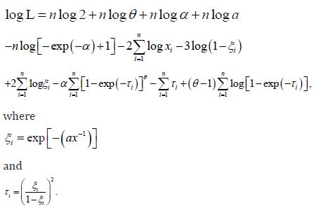
The score vector can be easily derived. Procedures of the method are available in the literature. Other estimation methods can be considered in other future works.
Modeling real data
We provide two applications to show empirically the potentiality of the PBXIE. In order to compare the fits of the PBXIE with other related distributions, we will consider the goodness-of-fit measures including the Akaike information criterion (AIC), Hannan-Quinn information criterion (HQIC), consistent Akaike information criterion (CAIC) and Bayesian information criterion (BIC), ,l− Cramér-von Mises ()*,W the Anderson-Darling ()*A and KS(p-value) statistics. These statistics are widely used to determine how closely a specific CDF fits the empirical distribution of a given data set. These statistics are given by
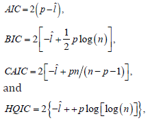
wherepis the number of parameters, n is the sample size and ˆl is the maximized log-likelihood.
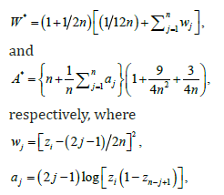
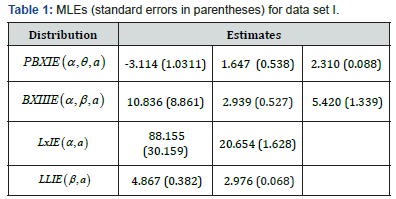
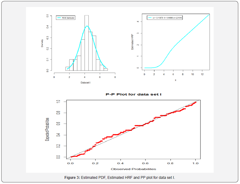
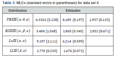
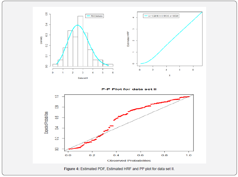
and ()iizFy= and the iy’s values are the ordered observations. The smaller these statistics are, the better the fit. The required computations are carried out using the R software. The MLEs and the corresponding standard errors (in parentheses) of the model parameters are given in Tables 1-4. The numerical values of the statistics *W and *A are listed in Tables 2 and 4. The histograms of the two data sets and the estimated PDF of the proposed model are displayed in Figures 2 and 3.

Application 1
The 1st real data set represents fracture toughness data given in Nadarajah & Kotz [2]. The data are: 5.5, 5, 4.9, 6.4, 5.1, 5.2, 5.2, 5, 4.7, 4, 4.5, 4.2, 4.1, 4.56, 5.01, 4.7, 3.13, 3.12, 2.68, 2.77,
2.7, 2.36, 4.38, 5.73, 4.35, 6.81, 1.91, 2.66, 2.61, 1.68, 2.04, 2.08, 2.13, 3.8, 3.73, 3.71, 3.28, 3.9,
4, 3.8, 4.1, 3.9, 4.05, 4, 3.95, 4, 4.5, 4.5, 4.2, 4.55, 4.65, 4.1, 4.25, 4.3, 4.5, 4.7, 5.15, 4.3, 4.5, 4.9,
5, 5.35,5.15, 5.25, 5.8, 5.85, 5.9, 5.75, 6.25, 6.05, 5.9, 3.6, 4.1, 4.5, 5.3, 4.85, 5.3, 5.45, 5.1, 5.3,
5.2, 5.3, 5.25, 4.75, 4.5, 4.2, 4, 4.15, 4.25, 4.3, 3.75, 3.95, 3.51, 4.13, 5.4, 5, 2.1, 4.6, 3.2, 2.5, 4.1,
3.5, 3.2, 3.3, 4.6, 4.3, 4.3, 4.5, 5.5,4.6, 4.9, 4.3, 3, 3.4, 3.7, 4.4, 4.9, 4.9, 5. Here, we shall compare the fits of the PBXIE distribution with those of other competitive models, namely the Burr IE (BXIIIE), Lomax IE (LxIE) and Log-logistic IE (LLIE) distributions (Tables 1&2).

Based on Table 4 and Figure 4 we note that the new lifetime model is much better than the all other considered competitive models.
Application 2
The 2nd real data set represents tax revenue data.
This data is given by: 3.7, 3.11, 4.42, 3.28,
3.75, 2.96, 3.39, 3.31, 3.15, 2.81, 1.41, 2.76, 3.19, 1.59, 2.17, 3.51, 1.84, 1.61, 1.57, 1.89, 2.74, 3.27,
2.41, 3.09, 2.43, 2.53, 2.81, 3.31, 2.35, 2.77, 2.68, 4.91, 1.57, 2.00, 1.17, 2.17, 0.39, 2.79, 1.08, 2.88,
2.73, 2.87, 3.19, 1.87, 2.95, 2.67, 4.20, 2.85, 2.55, 2.17, 2.97, 3.68, 0.81, 1.22, 5.08, 1.69, 3.68, 4.70,
2.03, 2.82, 2.50, 1.47, 3.22, 3.15, 2.97, 2.93, 3.33, 2.56, 2.59, 2.83, 1.36, 1.84, 5.56, 1.12, 2.48, 1.25,
2.48, 2.03, 1.61, 2.05, 3.60, 3.11, 1.69, 4.90, 3.39, 3.22, 2.55, 3.56, 2.38, 1.92, 0.98, 1.59, 1.73, 1.71,
1.18, 4.38, 0.85, 1.80, 2.12, 3.65.
Based on Table 4 and Figure 4 we note that the new lifetime model is much better than the all other considered competitive models (Tables 3&4).
Concluding Remarks
In this work, we derive a new inverse exponential continuous model via the zero truncated Poisson with a strong physical interpretation. A round of mathematical properties are derived. The maximum likelihood Method is considered for estimating the unknown parameter of our model. The new model is much better other important competitive models like Burr XII inverse exponential, Lomax inverse exponential and Log-logistic inverse exponential distributions.


