Mini Review

Longitudinal Data Analysis Using Liu Regression

Rahmani M¹, Arashi M¹* and Salarzadeh Jenatabadi H²

¹Department of Statistics, Shahrood University of Technology, Shahrood, Iran

²Department of Science and Technology Studies, University of Malaya, Malaysia

Submission: April 2, 2018; Published: July 18, 2018

*Corresponding author: Arashi M, Department of Statistics, Faculty of Mathematical Sciences, Shahrood University of Technology, Shahrood, Iran; Email: m_arashi_stat@yahoo.com

How to cite this article: Rahmani M, Arashi M, Salarzadeh J H. Longitudinal Data Analysis Using Liu Regression. Biostat Biometrics Open Acc J. 2018; 7(5): 555725. DOI: 10.19080/BBOAJ.2018.07.555725

Abstract

For understanding and characterizing discase progression over time, Eliot et al. [1] proposed a mixed ridge regression to account correlated outcomes and potentially high degree of correlated predictors for Biomarker data. However, the ridge estimator is non-linear in nature w.r.t. the ridge parameter and hence it is hard to estimate In this paper, we propose a linear unified approach to combat this difficultly. Numerical studies illustrate the usefulness of our approach compared to the mixed model.

Keywords: EM-algorithm; Liu regression; Longitudinal; Mixed model; Predictor variables; Design matrix; Regression coefficients; Predictive precision; Correlated predictors; Square root; T-distribution; Non-linear; Mixed model; Log-likelihood; Maximizing; Minimizing; Expectation-maximization; Algorithm; Real data analysis; Longitudinal data; Mean prediction error

Abbrevations: EDF: Effective Degrees of Freedom; EM: Expectation-Maximization; SD: Standard Deviation; MPE: Mean Prediction Error

Introduction

We begin with the simple linear regression model given by

Where, Y=(y₁,y₂,....,y_n) is an n×1 vector of responses, X is an np× design matrix comprised of p< n columns representing each of the potential predictor variables, n is the number of individuals in our sample and is an n×1 vector of independent errors. The least squares (LS)/maximum likelihood (ML) estimator of the regression coefficients is given by

and Notably, in the case that the columns of X are highly correlated, X^TX will be singular and we replace (X^TX)^-1 with (X^TX)^- where ‘-’ denotes the generalized inverse, and a unique solution to equation (1) does not exist. Further, in the case of high correlation where TXXis still invertible, the resulting coefficient estimates will have largely inflated variances, which in turn, results in low predictive precision.

Ridge regression, designed specifically to handle correlated predictors, involves introducing a shrinkage penalty λ to the least squares equation, and subsequently solving for the value such that

The solution to equation (2) is given by

and we have [2],

Further, dividing ˆβ by root n times the square root of its variance has a Student’s t-distribution with effective degrees of freedom (EDF) given by [3-5]. However, the ridge regression estimator ˆRβ is non-linear with respect to λ and its estimation is challenging. An alternative approach is proposed by Mayer & Willke [6]. The key idea is ˆdβ is closer to the true β for 0< d< 1 In section 2, we will develop their idea for longitudinal mixed model.

Linear mixed effects model

Now, consider the setting in which multiple measurements are observed for each individual over time. The mixed effects model for this setting is given by

Where, i=1,...,n represents individuals, is a vector of n_i observations for individual i, and X_i is the corresponding inp× design matrix of fixed effect covariates. We further assume are person-specific random effects, z_i is the corresponding random effects design matrix, and are independent random errors. Finally, we let Y,X and Z be appropriately defined matrices representing the concatenation of the corresponding variables over all individuals .i

The log-likelihood function of Y based on this model is given by

Where and iV is component corresponding to individual .i Maximizing this function with respect to the fixed effects parameter vector, β in the non-penalized setting is equivalent to minimizing the least squares objective function that gives the estimate of β as

Mixed-liu regression

In this section, we introduce a penalized regression approach to estimation for the mixed model given in equation (3). To begin, we assume the variance parameters θ=(σ,D) are known and add a penalization term to objective function of mixed model, which yields

Differentiating the objective function in equation (6), setting the resultant equal to 0 and solving, we have:

Hence,

We suggest to estimated in equation (7) by

We suggest to estimated in equation (7) by

Where

And

More generally, consider the setting in which the variance parameters θ=(σ,D) are unknown. Eliot et al. [1] proposed an extension of the expectation-maximization (EM) algorithm described by Laird & Ware [4], that includes an additional step for estimation of the ridge component. Here, we exhibit an EM algorithm to solve ˆMLiuβ for unknown .θ This approach is summarized by the following step-by-step procedure.

I. (E-Step) Initialize and Solve for and the sufficient statistics and given by:

II. (M-Step) Solve for where and n is the number of individuals in our sample, and let

IV. Repeat Steps (1)-(3) a large number of times and until a convergence criterion is met.

In the forthcoming section we evaluate the performance of the mixed Liu estimator by a Monte Carlo simulation study

Simulation study

A simple simulation study is conducted to characterize the relative performances of mixed Liu regression and the usual mixed effects modeling approach in the context of multiple, correlated predictors. For simplicity of presentation, the simulation study assumes repeatedly measured outcomes, while the predictor variables are measured at a single, baseline time point, as in Eliot et al. [1]. We further assume

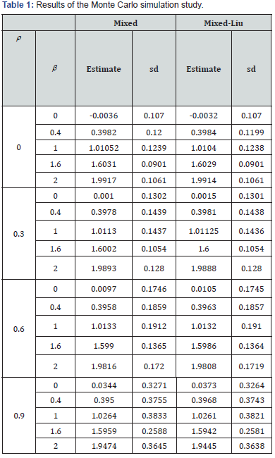
according to the model of equation(3) where β= (0,0.4,1,1.6,2), and Each predictor variable is assumed to arise from a normal distribution with mean equal to 5 and variance equal to 1. The correlation between predictor variables, given by ρ in Table 1, is assumed to take on values between 0 and 0.9. Starting values for the variance components are derived based on fitting a mixed model with no Liu component. In total, M=100 simulations are conducted for each condition based on sample sizes of n=40 individuals. According to the results of Table 1, the mixed Liu estimates often have lesser bias than the mixed ones. Also the mixed Liu is superior, in standard deviation (sd) sense.

Real data analysis

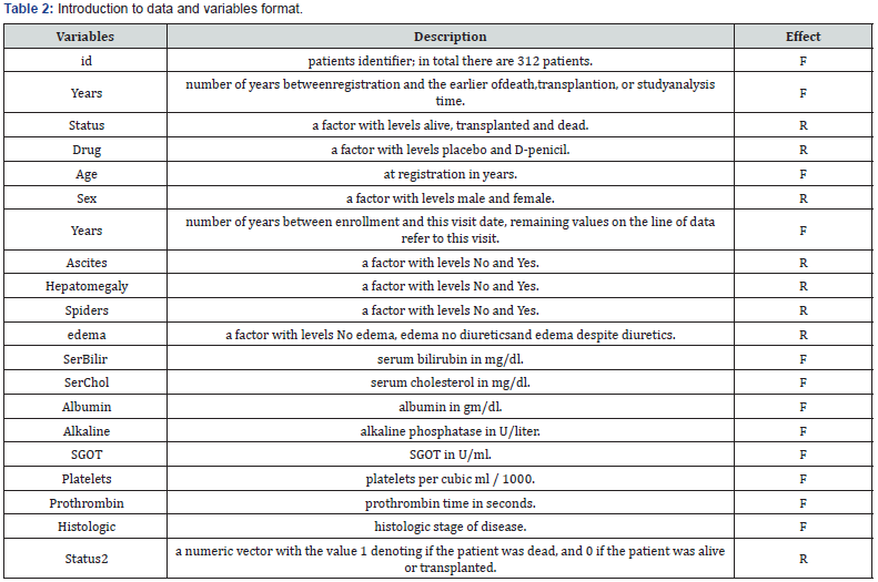
The data set we are analyzing here is the Mayo Clinic Primary Biliary Cirrhosis data, from the package “JMbayes” in R software. It consists of 312 randomized patients with primary biliary cirrhosis, a rare autoimmune liver disease, at Mayo Clinic. In this study we have 1945 observations on the 20 variables, listed in Table 2. The response variable is the number of years, indicated as “years” in Table 2 and the variables considered as fixed and random effects are marked as “F” and “R”, respectively in this table. Since the variables have been measured number of times for each individuals, so we have a longitudinal data set. On the other hand, some of the variables like sex in this data set will put the subjects in special groups, so we can consider these variables as random effects, as marked as “R” in Table 2, so we should use mixed model for analyzing this data set. The estimate of coefficients are obtained using the EM algorithm as outlined in Section 2. To compare the performance of the mixed Liu estimator, we evaluate the mean prediction error (MPE); the lesser, the better. In what follows, we describe the scheme we used to derive the MPE.

For our purpose, a K- fold cross validation is used to obtain an estimate of the prediction errors of the model. In a K-fold cross validation, the dataset is randomly divided into K subsets of roughly equal size. One subset is left aside, {(X^Test,Y^Test)} termed as test set, while the remaining 1K− subsets, called the training set, are used to fit model. The resultant estimator is called ˆ.trainβ The fitted model is then used to predict the responses of test data set. Finally, prediction errors are obtained by taking the squared deviation of the observed and predicted values in the test set, i.e.

Where The process is repeated for all K subsets and the prediction errors are combined. To account for the random variation of the cross validation, the process is reiterated N times and is estimated the average prediction error is given by

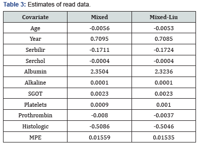
Where PE^k_N is the prediction error of considering kth test set in ith iteration. Our result are based on N=200 case resampled bootstrap sample. In Table 3, we report the estimates and MPE values. Based on the results, the proposed mixed-Liu estimator performs better than the mixed one, in MPE sense. Further, the absolute value of estimates in the mixed Liu estimates are lesser than the mixed.

Conclusion

In this paper, we developed a linear unified procedure called Liu in the linear mixed model for longitudinal data analysis. Hence, we considered a penalized likelihood approach and propose the Liu-mixed regression estimator for the vector of regression coefficients. An EM algorithm also exhibited to solve the penalized likelihood for the unknown parameters. Numerical studies demonstrated the good performance of the proposed mixed Liu estimator for the multicollinear situation.

References

1. Eliot M, Ferguson J, Reilly MP, Foulkes AS (2011) Ridge Regression for Longitudinal Biomarker Data. Int J Biostat 7(1): 37.
2. Hoerl A, Kennard R (1970) Ridge regression: Applications to nonorthogonal problems. Technometrics 12: 69-82.
3. Hoerl A, Kennard R (1970) Ridge regression: Biased estimation for nonorthogonal problems. Technometrics 12: 55-67.
4. Laird N, Ware J (1982) Random-effects models for longitudinal data. Biometrics 38(4): 963-974.
5. Malo N, Libiger O, Schork N (1982) Random-effects models for longitudinal data. Biometrics 82: 375-385
6. Mayer LS, Willke IA (1973) On biased estimation in linear model. Technometrics 15: 497-508.