


Limits and Inferences for Alpha-Stable Variables
Jensen DR
Department of Statistics, Virginia Polytechnic Institute and State University, USA
Submission: October 05, 2017; Published: December 8, 2017
*Corresponding author: DR Jensen, Emeritus Professor, Department of Statistics, Virginia Polytechnic Institute and State University, Blacksburg, VA 24061, USA, Tel: 540-639-0865; Email: djensen@vt.edu
How to cite this article: Jensen DR. Limits and Inferences for Alpha�Stable Variables. Biostat Biometrics Open Acc J. 2017; 4(1): 555630. DOI: 10.19080/BBOAJ.2017.04.555630
Abstract
Distributions having excessive tails are modeled in various venues via a-stable sequences deficit in moments of various orders. Essential statistics are examined under independent vs spherically dependent cases. The former exhibits such critical pathologies as inconsistent sample means. The latter support versions of some classical procedures even without moments as conventionally required. In particular, despite heavy tails, Student's tests for means nonetheless remain exact in level and power. etc. AMS Subject Classification: 62E15, 62H15, 62J20.
Keywords: Excessive tails; α- stable sequences; Consistency; Exact Student's t
Introduction
Classical statistics rest heavily on means, variances, correlations, skewness and kurtosis, requiring moments to fourth order. To the contrary, probability distributions having excessive tails, often void of first or second moments, arise in a variety of circumstances. These encompass radar tracking, image processing, acoustics, risk management, portfolios in finance, biometrics, and other venues. Supporting references include Bonato & Matteo [1], Cheng & Rachev [2], Kim et al. [3], Kuruoglu & Zerubia [4], Qiou et al. [5], Tsionas & Efthymios [6]. Salient monographs are Arce [7], Chernobai & Rachev [8], Ibragimov et al. [9], and Samorodnitsky & Taqqu [10]. In these settings the classical foundations accordingly must be reworked.
Excessive tails typically are modeled through α- stable distributions with index α∈[0,2]. These comprise all limit distributions for standardized partial sums, of which Gaussian central limit theory applies under second moments with α = 2 Despite the circumstances cited, usage has been limited for want of explicit expressions, apart from special cases, for α-stable density and cumulative distribution functions. Nonetheless, signal progress is supported through the use of characteristic functions (chfs). as undertaken in this study. Even here a divide emerges between independent, identically distributed (iid) α-stable variables, or dependent α-stable (sαs)sequences. An outline follows. Notation and technical foundations are provided in Section 2. The findings in Section 3 are twofold: First, that limit properties diverge widely between (iid) and spherically dependent (sαs) sequences; and second, that conventional inferences, though largely lacking in the former, may be validated in large part in the latter. Conclusions are tallied in Section 4.
Preliminaries
Notation: Spaces include ℝN as Euclidean N-space. Vectors and matrices are set in bold type; the transpose, inverse, trace,and determinant of A are A', A-1, tr(A), and |A| the unit vector in ℝN is 1N = [1,...., 1]'; and IN is the (N x N) identity. Moreover, Diag (A1.......Ak) is a block-diagonal array.
Special distributions
For Y=[Y1,...,YN]' ϵℝN, its distribution, mean, and dispersion matrix are denoted by L(y),E(y) =μ and v(y)=Σ, say, with variance var(y) = σ2 on 1 ℝ1. Specifically, L(Y)=NN(μΣ) is Gaussian on ℝN with parameters (μ,Σ). Distributions on ℝ1 include the χ2(μ;v,λ) having degrees of freedom and non centrality parameter λ; and the corresponding Student's t2(μ;v,λ). The (chfs) for Y is the expectation ϕY(t)=E[eit'Y] with argument t' = [t1,........tN]; a standard source is Lukacs & Laha [11]. Reference is drawn subsequently to probability density (PD) and cumulative distribution (CD) functions.
Foundations
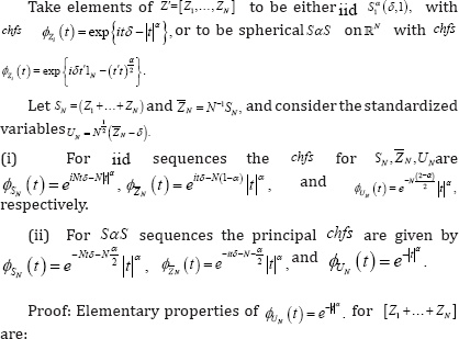
A random process ℤ={Zt;tϵτ} is spherically invariant if for each N , the joint (chfs) of [Z1,...,ZN] has the form ϕz(t)=Ψ(t't) for some function Ψ(.) not depending on N [12,13]. Averages and limits are basic in statistical analysis; for example, notions of consistency in estimation and of large-sample distributions. These are undertaken here without benefit of moments in keeping with excessive tails. Specifically, the sequence ℤ={Zt;tϵτ} supplies the context for taking limits. In addition, the following is central to this study, where[δ,ε] respectively comprise a location vector and a matrix of scale parameters, the latter taking the value Σ;=INin the case of spherical symmetry on ℝN
Definition 1: L(Z)ϵ SNα(δ,Σ) designates an elliptical α-stable law on ℝN centered at δϵℝN with scale parameters Σ and stable index αϵ(o,2], having the (chfs) ϕZ(t)=exp{it'δ-(t'Σt)α/2} Each marginal distribution of SNα(δIN onϵ1 namely S1α(δ,1), has the(chfs) ϕZt(t)= exp {itδ-/t/α}
Remark 1: For αϵ(0,2) these have moments of order up to but excluding α but with moments of all orders at α = 2. Included are elliptical Cauchy and Gaussian laws at α = {1,2}, respectively. In addition, the following is central to subsequent developments.
Lemma 1: Let gN(z;δ,In) be the density for NN(δ,σ2,In and fαN(z;δ,In)the SαS density for L(Z)ϵSαN(δ,In). Then therechfs and pdfs are related as follows.
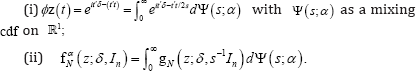
Proof: Hartman & Wintner [12] gave a necessary and sufficient condition that the process  be spherically invariant, namely, that for each N
  the chfs ϕZ(t) is a scale mixture of N-dimensional spherical Gaussian chfs. This applies in context to give conclusion (i). To continue,
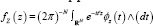 is the standard inversion formula from chfs to densities with ^(.) as Lebesgue measure. Accordingly, we invert both sides of the second and third expressions in conclusion (i) to get the density on the left of conclusion (ii). We then recover the right side of conclusion (ii) on reversing the order of integration in the iterated integral found on inverting the third expression of conclusion (i).
The Principal findings
Sequences of iid and SαS Variables: Much of classical statistics rests on iid random variables. In the present context it is germane to ask whether spherical SαS Variables [Z1,....,ZN] might also be independent. To the contrary, for any spherical sequence. Maxwell [14] showed this to be the case if and only if Gaussian. In view of this, it remains to examine the limit properties of iid SαS Variables in comparison with spherically dependent SαS Variables in ℝN of critical interest to users. Limit properties of these are shown next to be widely disparate, despite the fact that their marginals coincide. At issue are statistics 
 in order to be iid. A principal finding follows.
I.Theorem 1
a. If independent, then 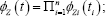
b. The chfs of SN is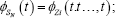 and
and
c.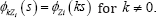
Conclusions (i) and (ii) follow directly from these. Developments to follow invoke the following principles, first for iid and then for spherical SαS sequences.
Remark 2: In the chfs 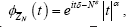 note that
 factors in as a scale parameter. For consistency in estimatingS,δ it is necessary and sufficientthat
 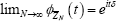 which, by the Levy-Cramer continuity theorem, is the chfs of a distribution degenerate at δ Consistency of
  for then follows using the equivalence of convergence in law to degeneracy, and convergence in probability.
II.Theorem 2
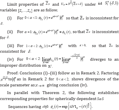
III. Theorem 3
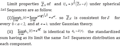
Proof: Conclusion (i) follows from the second chfs of Theorem 1(ii) as in Remark 2, and conclusion (ii) directly per se from the third chfs of Theorem 1(ii). In short, it is seen from Theorem 2 that iid α-stable variables hold little promise to exhibit even basic properties in data analysis and statistical inference, where even the consistency of δ for requires knowing that 1 2. On the other hand, the next section motivates circumstances for the occurrence of spherical sas samples, and sets out to establish useful statistical properties in the analysis of data from these models.
Properties of spherical SαS samples
Consider anew a single sample with parameters (δ,σ2), taking 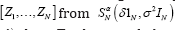 in lieu of the conventional iid Nt(δ,σ2) data. To these ends
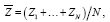 and identify
  as the ordinary residuals, with
  as the projection onto the error space, and
  . Recall that the two-sided normal-theory test for
  uses the conventional Student's
  The following is central to our findings.
IV. Theorem 4
Given that  we seek the joint distribution of
 and that of
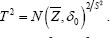 .
.
(i) The joint distribution of  is given by
 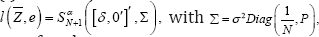 a distribution ℝN+1 on of rank N.
(ii) The marginals are centered  at δ with scale parameter
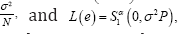 the latter a distribution on ℝN of rank n-1 centered at 0 with scale parameters σ2p
(iii) has density
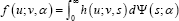 with h(μv,s)
as the scaled central chi-squared density having v=(N-1)degrees of freedom, and with s;a) as a mixing distribution from Lemma 1.
with h(μv,s)
as the scaled central chi-squared density having v=(N-1)degrees of freedom, and with s;a) as a mixing distribution from Lemma 1.
(iv) The test for  is exact in level and power as its normal - theory version, for all
Proof: Take Its  chfs with argument
is  with argument V=H's replacing t
Conclusion (i) follows on substituting into to give
 since p is idempotent, so that
 as claimed.
Conclusion (ii) follows directly.
Conclusions (iii) and (iv) attribute to Hartman & Wintner[12] through Lemma 1(ii). Specifically, a change of variables μ→e→S2 behind the integral on the right of Lemma 1(ii) gives the conditional density for L(S2\s) namely the scaled chi-squared density h(μv,s) depending on s, so that integrating with respect to dΨ(s;α) as in Lemma 1(ii) gives conclusion (iii). In like manner, the change of variables 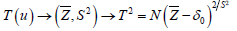 behind the integral in Lemma 1(ii) gives the conditional density for L(T2\s) But this statistic is scale-invariant and thus independent of the mixing distribution Ψ(s;α) so that L(T2\s)=L(T2)unconditionally, the latter being its conventional normal-theory distribution
Remark 3: Despite the diagonal structure  in conclusion (i), (Ž,e) are independent if and only if Gaussian at α = 2 on applying Maxwell’s (1860) result. The mixtures of Lemma 1 and their consequences deserve further mention. Given l(y) L(Y)=N
Corollary 1: Consider 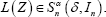 The Cauchy chfs and density functions at α = 1 may be represented as follows.
(i) 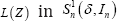 has the mixing distribution
 at v=1 namely, the chi-distribution with density
 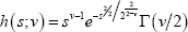 having of freedom
(ii) Beginning with  the spherical Cauchy density is
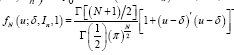
Proof: The conclusions follow on specializing the mixing distribution for the multi variate t at v=1 degree of freedom, and its known density at v =1
Conclusion
In practice scale mixtures may arise as conditionally iid Gaussian variables subject to scaling in a random environment. Linear models so structured are treated in Zellner [15] under multivariate Student t in lieu of Gaussian errors. The present study complements that work, eschewing moments through spherical Cauchy errors having v =1 degree of freedom. In summary, we have modeled errors not as iid, but instead as spherical α-stable errors. The former holds little promise as noted, where even the consistency of for δ requires that 1 <α≤2, yet α typically is unknown. On the other hand, spherical α-stable errors offer a reasonable resolution to open topics in linear inference without moments. Not only is consistent for δ for all αϵ(o,2], but a mixture representation is given for the density of S2/σ2 Moreover, a corresponding representation for Student's T2 exploits its scale invariance to show that tests using T2 are exact in level and power, as for Gaussian errors, for all L(Z)=SNα(δ1N,σ2IN) with 0 ≤ α ≤2.
References
- Bonato M (2012) Modeling fat tails in stock returns: A multivariate stable-GARCH approach. Computational Statist 27(3): 499-521.
- Cheng BN, Rachev ST (1995) Multivariate stable futures prices. Mathematical Finance 5(20: 133-153.
- Kim YS, Glacometti R, Rachev ST, Fabozzi FJ, Mignacca D (2012) Measuring financial risk and portfolio optimization with a non- Gaussian multivariate model. Ann Operations Research 201: 325-343.
- Kuruoglu E, Zerubia J (2009) Modeling SAR Images with a generalization of the Rayleigh distribution. IEEE Trans. Image Processing 13(4): 527533.
- Qiou Z, Ravishanker N, Dey DK (1999) Multivariate survival analysis with positive stable frailties. Biometrics 55(2): 637-644.
- Tsionas EG (2012) Estimating multivariate heavy tails and principal directions easily, with an application to international exchange rates. Statist and Probability Letters 82(11): 1986-1989.
- Arce GR (2000) Nonlinear Signal Processing. Wiley, New York.
- Chernobai A, Rachev ST, Fabozzi FJ (2007) Operational Risk: A Guide to Basel II Capital Requirements, Models and Analysis. Wiley, New Jersey, USA.
- Ibragimov M, Ibragimov R, Walden J (2015) Implications of heavy tailedness. In: Heavy-Tailed Distributions and Robustness in Economics and Finance (1st edn). Lecture Notes in Statistics, 214. Springer-Verlag, Berlin, Germany.
- Samorodnitsky G, Taqqu M (1994) Stable Non-Gaussian Random Processes. Chapman and Hall, New York.
- Lukacs E, Laha RG (1964) Applications of Characteristic Functions. Hafner, New York, USA.
- Hartman P, Wintner A (1940) On the spherical approach to the normal distribution law. Amer J Math 62(1): 759-779.
- Kelker D (1970) Distribution theory of spherical distributions and a location scale parameter generalization. Sankhya 32(4): 419-430.
- Maxwell JC (1860) Illustrations of the dynamical theory of gases. Part 1: On the motion and collisions of perfectly elastic spheres. Philosophical Mag 19(1860): 19-32.
- Zellner A (1976) Bayesian and non-Bayesian analysis of the regression model with multivariate Student-t error terms. J Amer Statist Assoc 71(1976): 400-405.


