ASPEN Study Case: Real Time in Situ Tomato Detection and Localization for Yield Estimation
Camilo Chiang1,2*, Daniel Tran1 and Cedric Camps1
1Agroscope, Institute for Plant Production Systems, Rue de eterpys 18, 1964 Conthey, Switzerland
2Agroscope, Digital Production, Tänikon 1, 8356 Ettenhausen, Switzerland
Submission: March 13, 2024; Published: March 21, 2024
*Corresponding author: Camilo Chiang, Agroscope, Institute for Plant Production Systems, Rue de eterpys 18, 1964 Conthey, Agroscope, Digital Production, Tänikon 1, 8356 Ettenhausen, Switzerland
How to cite this article: Camilo C, Daniel T, Cedric C. ASPEN Study Case: Real Time in Situ Tomato Detection and Localization for Yield Estimation. Agri Res& Tech: Open Access J. 2024; 28(3): 556406. DOI: 10.19080/ARTOAJ.2024.28.556406
Abstract
As the human population continues to grow, our food production system is challenge. With tomato as the main fruit produced indoors, the selection of varieties adapted to specific conditions and higher yields is an imperative task if we are to meet the growing food demand. To assist growers and researchers in the task of phenotyping, we present a study case of the Agroscope phenotyping tool (ASPEN) in tomato. We show that when using the ASPEN pipeline, it is possible to obtain real-time in situ yield estimation without a previous calibration. To discuss our results, we analyse the two main steps of the pipeline in a desktop computer: object detection and tracking, and yield prediction. Thanks to the use of YOLOv5, we obtain a mean average precision for all categories of 0.85, which together with the best multiple object tracking (MOT) tested allow obtaining a correlation value of 0.97 compared to the real number of tomatoes harvested and a correlation of 0.91 when considering the yield thanks to the use of a SLAM algorithm. In addition, the ASPEN pipeline demonstrated to be able of predicting subsequent harvests. Our results demonstrate in situ and real-time size and quality estimation per fruit, which could be beneficial for multiple users. To increase the accessibility and use of new technologies, we make publicly available the necessary hardware material and software to reproduce this pipeline, which includes a dataset of more than 820 relabelled images for the tomato object detection task and the trained weights
Keywords: Tomato; Yield; Food production system; Phenotyping; Agricultural industry; Fruit detection
Abbreviations: MOT: Multiple Object Tracking; UGV: Unmanned Ground Vehicles; NN: Neutral Networks; LIDAR: Light Detection and Ranging; SFM: Structure from Motion; SLAM: Simultaneous Localisation and Mapping; ASPEN: Agroscope Phenotyping Tool; CNN: Convolutional Neural Network; GUI: Graphical User Interface; GFLOPS: Giga Floating-Point Operations Per Second; ROI: Region of Interest; RSE: Residual Standard Error
Introduction
As we approach the estimated inflection point of the world population growth curve UN, increasing global food availability is more important than ever. Especially with the current climate crisis threatening our food system Owino et al. [1]. Several strategies have been applied throughout the food production chain to address this issue FAO [2]. To this end, new methods have been tested across the agricultural industry to speed up results and increase efficiency, particularly in new technologies in a so-called fourth agricultural revolution, even though the impact of these new technologies is not clear Barret & Rose [3]. The vast majority of these new methods require large amounts of information obtained directly from the field or plants, in descriptive processes called phenotyping. Phenotyping is the activity of describing, recording or analysing the specific characteristics of a plant and due to the nature of this process and the required frequency, it is a time-consuming task Xiao et al. [4]. While the principle of phenotyping is not new, the quantity and quality of information that is today been generated has never been seen before, making imperative to reduce the time required for this task. Remote sensing has been used and its automation has already been demonstrated thanks to new algorithms and technologies Chawade et al. [5], even further opening up new opportunities for real-time data utilisation, what could save resources and further improve the industry as a whole Bronson & Knezevic [6].
There are several ways to automate phenotyping, with each path depending on the allocated budget and working conditions. For example, Araus et al. [7] divide these paths according to the distance to the target. Satellites can be used with fast data acquisition per m2, but with a trade-off between resolution and investment costs. Other methods closer to the plants, such as stationary platforms, allow for higher spatial resolution data, but are less flexible and more expensive to implement. A proven solution is the use of drones, which are more flexible than fixed platforms, but still not as flexible as they cannot work in covered crops. On the other hand, handheld sensors, manned or unmanned ground vehicles (UGVs) are more flexible than the aforementioned platforms and have a higher resolution, a lower initial investment, but can cover smaller areas than the previously mentioned methods. The effectiveness of this last category has been well demonstrated, especially in the fruit detection and localisation tasks e.g. Scalisi et al. [8], but affordable open-source alternatives are scare. The phenotyping subtask of fruit detection in images was initially based on shape and colour, until the advent of neutral networks (NN), which were particularly advanced after 2012 e.g. Hinton et al. [9]. These have led to more robust results in fruit detection.
Today, well-established algorithms such as RCNN Girshick et al. [10], Mask-RCNN He et al. [11] and YOLO Redmon et al. [10] are constantly used for research purposes and in production environments. For example, Mu et al. [12] show that when using RCNN, they could achieve a mean average precision at 0.5 intersection over union (IoU) (mAP@0.5) of 87.63%, which later correlates with the real number of tomatoes per image at 87%. Other authors, Afonso et al. [13]; Seo et al. [14]; Zu et al. [15] showed that when using Mask-RCNN, focused on the task of instance segmentation, they obtain a similar or higher average precision than Mu et al. [12], with values of mAP up to 98%, 88.6% and 92.84% respectively in each study. These previous works demonstrate the ability of the presented algorithms not only to detect objects, but especially to detect individual tomatoes in situ. A notable point of these works is that the comparability of their results is technically incorrect since each detection algorithm was trained on different image datasets. To compensate for this, a standardised dataset must be used and although some few datasets are freely available online to train machine learning algorithms in the task of tomato object detection, these are rarely used. Remarkable datasets are "laboro tomato" Laboroai [16] and "tomatOD" Tsironis et al. [17] due to its quality and availability.
Although the previously mentioned NN based algorithms have good detection rates, they are not capable of running in real time (more than 30 frames per second, FPS). For example, using a variant of R-CNN, Faster R-CNN, Seo et al. [14] achieve up to 5.5 FPS using a desktop computer equipped with a graphics processing unit (GPU) card (NVIDIA GTX 2080 ti), without mentioning the input size of the model. Thanks to the introduction of YOLO, Liu et al. [18] have shown that near real-time analysis is possible. In their case, the authors improved the YOLOv3 model by using a denser architecture and round boundary boxes that better fit the shape of tomatoes. These changes allowed them to achieve an F1 score, a weighted average of precision and recall, of 93.91% at a speed of 54 ms (18 FPS), compared to 91.24% at 45 ms (22 FPS) and 92.89% at 231 ms (4.3 FPS) for the original YOLOv3 and Faster R-CNN, respectively. In their case, images of 416x416 pixels were processed on a desktop computer equipped with a GPU (NVIDIA GTX 1070Ti). With a faster, more robust and more recent version of YOLO, YOLOv5, Egi et al. [19] achieve an F1 score of 0.74 for red tomatoes, which correlates at 85% with a manual count. Although no speed was documented in their work, the various algorithms of YOLOv5 are capable of running in real time at resolutions below 1280 pixels, depending on the system used (CPU vs. GPU) and model implementation Jocher et al. [20]. In addition, Egi et al. [19] demonstrate that the use of a state-of-the-art multiple object tracking (MOT) algorithm allows each individual object to be tracked along a video sequence.
For the tracking task, several MOT algorithms have been proposed, among which we highlight SORT Bewley et al. [21], bytetrack Zhang et al. [22] and OCSORT Cao et al. [23] as their code is publicly available, they have a high performance and they can run in real time in a common CPU unit even in the presence of multiple objects. Once an object has been detected, it needs to be located in space, which can be done in a number of ways. One simple way is to use RGBD cameras that contain a deep channel (D). This information can be used to distinguish the foreground from the background objects, which has been well demonstrated in tomatoes by Afonso et al. [13], allowing for object localization within frame, but missing the global position of the detected objects. Using an alternative methodology, Underwood et al. [24] show that it is possible to reconstruct a non-structural environment using Light Detection and Ranging (LiDAR) technology for within frame, together with GPS data for global localization in a post-processing method. Thanks to their method, they were able to locate and estimate almond yield at tree level with an R2 of 0.71.
The use of 3D reconstruction techniques has been less explored in greenhouses. Masuda et al. [25], show that tomato point clouds obtained from structure from motion (SfM) can be further analysed to obtain per plant parameters such as leaf area, vapour length using a 3D neutral network, Pointnet++ Qi et al. [26], with an R2 of 0.76 between the ground truth area and the corresponding number of points.
In a more advanced analysis, Rapado et al. (2022) show that by using a 3D multi-object tracking algorithm, that really in an RGB camera and LiDAR, they achieve a maximum error of 5.08% when localising and counting tomatoes at a speed of 10 FPS. Similarly, other authors have documented that by the year 2022, pipelines based on existing 3D neural networks are slower than 2D methods that really in additional sensors to obtain deep information (e.g. Afonso et al. [13], Ge et al. [27]. In addition, actual 3D neural networks have major limitations such as maximum input size, large number of parameters that make them slower to train, high memory consumption, and moreover, they are particularly limited by the lack of datasets for training reasons Qi et al. [28].Nevertheless, new low-cost 3D pipelines and datasets are constantly being released to increase the availability of this technology (e.g. Schunck et al. 2022, Wang et al. [29].
In order to correlate these detections with real yields, 3D localisation is required, and remarkably, simultaneous localisation and mapping (SLAM) algorithms have not been widely used in agricultural environments, possibly due to their lack of robustness Cadena et al. [30]. Previous SLAM methods are suitable for more structured environments, with clear corners and planes that allow incoming LiDAR scans to be aligned, which can be used for localisation (LiDAR odometry, LIO). A possible solution for unstructured environments is to use images for localisation (visual odometry, VIO), but this tends to fail in fast motion. Sensor fusion, a technique that fuses multiple sensors together, can provide more robust systems that can, for example, align incoming LiDAR scans when using VIO for navigation. This technology is better suited to environments that lack clear features, such as outdoor environments. Notable examples of these algorithms due its robustness and open source code include VINS-FUSION Qin et al. [31], CamVox Zhu et al. [32], R3Live Lin & Zhang [33], and FAST-LIVO Zheng et al. [34].
The low use of these technologies in the agricultural sector, either separately or together, could be attributed to several reasons, including the maturity of the technologies, budgetary reasons, and a knowledge gap between farmers and computer science e.g. Kasemi et al. [35]. The Agroscope Phenotyping Tool (ASPEN) aims to break the digital phenotyping barrier among agricultural researchers, thanks to a proven and affordable pipeline that can work in situ and in real time for fruit detection, allowing non-experts to use the tool. In this paper, we demonstrate that this pipeline: 1) allows 3D reconstruction of a non-structured environment using a SLAM algorithm, and thanks to this 2) can localise and describe tomato fruits in a traditional greenhouse thanks to the addition of an object detection algorithm. Most importantly, in order to increase the accessibility and use of this pipeline, we are making the necessary hardware and software to reproduce it publicly available, which we hope will help to bridge the gap between agricultural and computer scientists.
Materials and Methods
Hardware and Software
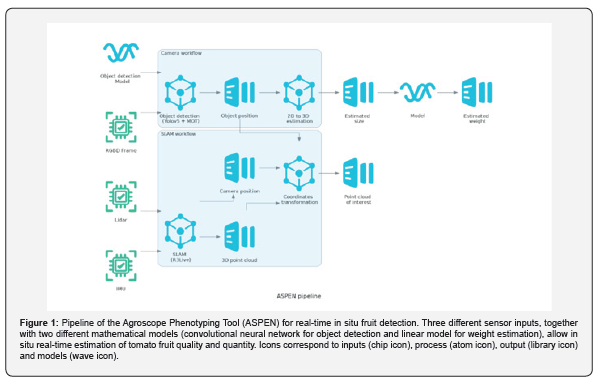
An ASPEN unit was used to evaluate the ASPEN pipeline (Figure 1). Although it is not the aim of this paper to discuss the configuration or selection of the equipment used, a brief description is given below. For more details, the reader is invited to refer to the online project repository (https://github.com/camilochiang/aspen, Chiang et al. in preparation). The ASPEN pipeline considers a set of input sensors connected to an embedded computer using the robot operating system (ROS, Stanford Artificial Intelligence Laboratory et al. 2018), version melodic in a gnome-based version of Ubuntu 18.04.6 LTS, with the aim of reconstructing and locating plants, fruits or diseases in situ in real time, where we here focus in the fruit case. ASPEN uses a specific selection of sensors and electronic components that may already be present in an agricultural research facility. To achieve this goal, the system relies on two main workflows, tightly coupled and orchestrated by an embedded computer equipped with a GPU (Jetson Xavier NX 16 Gb): the camera workflow and the SLAM workflow.
For the camera workflow, a synchronised RGBD without timestamp synchronisation (Realsense, R415 - 1920x1080 pixels at 30 FPS with synchronised depth) is processed with a convolutional neural network (CNN) object detection technique based on the RGB. Once that a model has been selected and object detection per frame has been performed, each object is identified and tracked using a multi-object tracking (MOT) algorithm were an unique ID is assigned. Finally, once the detected tracked object passes a region of interest (ROI) of the field of view and it is confirmed as a unique object who have not been register before, its localisation within the image is transferred to the 2D to 3D estimation node. Using the localisation given by the MOT algorithm for each object, the 2D to 3D estimation node uses the deep (D) frame information to estimate the dimensions (mm) of the tracked object and its localization with respect the camera position. For each object detection, the minimum distance to the camera is extracted and then the actual diameter is calculated and used by a dimensional model (Figure 1) to convert to weight (g).
In addition to this workflow, two other sensors, an Inertial Measurement Unit (IMU, BMI088 bosh) and a Light Detection and Ranging (LiDAR, Livox mid-70, configured into single return mode) unit, as well as the RGB channels of the RGBD camera, are used in the parallel SLAM workflow who allow to locate each RGBD frame within a global mapping and therefore each tracked object in a 3D map. These sensors were choose due its low cost compared with similar sensors, and in case of the LiDAR especially due the extreme low minimum detection range (5 cm). The aim of this workflow is to reconstruct the environment in which the tomatoes are located and to provide a relative position for each tomato (with respect to the initial scanning point), which will then allow the detected tomatoes to be correlated with the handmade measurements. For this task, R3Live Lin & Zhang [33] was chosen as the SLAM algorithm, as it attaches new incoming points from the LiDAR unit (10 Hz) using the IMU (200 Hz) and image information and does not really only use LiDAR features for this task and can run in real time (faster than 30 FPS). These characteristics, shared with other similar visual odometry algorithms (VIO), show in our preliminary research to work better in agricultural environments in collaboration with SLAM algorithms that rely only in LiDAR odometry (LIO) (data not shown), potentially due to the clear lack of features (corners, planes) in a so-called "unstructured environment", which makes LIO algorithms more difficult to converge. To allow reproducibility, the input from all sensors are recorded within the ASPEN unit. A simple graphical user interface (GUI) is available to facilitate this task.
Experiments
To evaluate the ASPEN pipeline in the specific task of tomato detection and localisation, we started by training YOLOv5. Five different models (n, s, m, l and x) from the YOLOv5 family were trained at two different resolutions: 512 (batch size 20) and 1024 (batch size 6) pixels up to 300 epochs. These models differ mainly in the complexity of the model architecture, with the simpler models aiming to operate under resource-constrained conditions, such as mobile phones and embedded computers. This network was trained using 646 images for training and 176 images for validation, coming from our own datasets and other open source datasets (laboro-tomato and tomatoD). Regardless of the origin of the dataset, tomatoes were re-labelled in three different categories: immature, turning and mature tomatoes, with approximately 3500, 1000 and 900 instances of each category, respectively. After training, one of the resolutions and one of the models were selected for a posteriori use. For details of the dataset, the reader is invited to visit the online repository.
Once the model that met our requirements and had the best performance had been selected, two commercial-type greenhouses in the facilities of Agroscope (Conthey, Switzerland), with tomatoes of the Foundation variety grafted on DRO141, were scanned with an ASPEN unit on three consecutive harvest days in the middle of the production period of 2022. Each scan lasted a maximum of 12 minutes and was performed close to midday to ensure similar light conditions. Each greenhouse of approximately 360 m2 contained eight rows of tomato plants, each row 25 m long. The six central rows were scanned sequentially, with both sides of each row scanned before moving on to the next row. These rows were also divided into 3 blocks for other experiments, with buffer plants at the beginning, between blocks and at the end of each row. The scans were recorded as bag files using ROS. The resulting bag files were then transferred to a desktop computer (Lenovo ThinkPad P15, Intel core i9, GPU NVIDIA Quadro RTX 5000 Max-Q, 16VGb) for reproductive and posterior analysis. The analysis was automated with the aim of detecting tomatoes per block. To do this, the videos were first reviewed and pre-registered with timestamps of the transition between blocks.
To validate our results, after each scan we harvest all the tomatoes ready for marketing. Harvesting was done per bunch, usually from 4 to 5 tomatoes, which occasionally led to the harvesting of turning tomatoes. Harvesting took place either on the same day or the following day after each scan. To increase the spatial resolution of the validation data, each row was harvested side-by-side and each row was further divided into three different blocks, resulting in 216 validation points. This was incorporated into the analysis using a distance filter with the D-frame of the RGBD camera, ignoring any objects detected more than 50 cm from the ASPEN unit, as these correspond to elements in the background or on the other side of the row. For each harvest, the total weight was measured, including the weight of the pedicel. Differently, the number of fruits was counted per block only, regardless of the side of the row, giving 108 validation points. To build the size-to-weight model shown in Figure 2, after each scan, 100 tomatoes were harvested from the non-scanned rows belonging to the three categories mentioned above. These tomatoes were measured and weighted, and the model used later for yield estimation is shown in Figure 3.

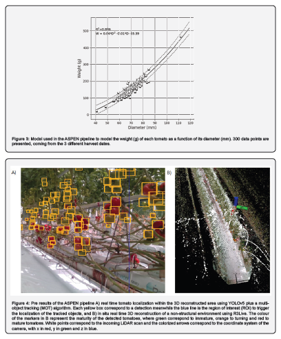
To complement the validation of the ASPEN pipeline, three MOT algorithms were tested under similar implementation frameworks and parameters (Python 3.8): SORT Bewley et al. [21], Bytrack Zhang et al. [22], and OCSORT Cao et al. [23].The quality of the yield estimation results depends not only on good object detection, but also on correct tracking along the frames until each object reaches a region of interest (ROI), where it is counted. Independently of the MOT algorithm used, an estimated position, size and weight was calculated for each tomato detected. An example of the detection and reconstruction process is shown in Figure 4. The correlation of the three different MOT algorithms with weight and count in relation to the real harvest is shown in Figure 5.

Statistics
A priori and posteriori statistical analyses were performed using Python 3.8 Van Rossum & Drake [36] and the Statsmodels package (version 0.13.5, Seabold & Perktold [37]. A quadratic equation was fitted to the size-weight relationship (Figure 3), as this statistically fit the data better than a simpler relationship (data not shown). To estimate the correlation between crop yields, either in number or weight, a linear correlation without intercept was fitted between the manually measured data and the estimated data from the ASPEN pipeline, considering each crop subsample as a data point (n = 108 for the number task and n = 216 for the weight task). To evaluate the ability of the ASPEN pipeline to predict future yields based on previous measurements, we correlate the estimated number of tomatoes in the turning category with the following 3 harvests for each subsample as a data point (n = 108). Finally, to evaluate the task of size measurement, an f test of the size distribution was carried out within each category (Figure 6).
Results
Object detection
Within the ASPEN pipeline, the first task in the camera workflow is object detection (Figure 1), which requires a previously trained object detection model. As shown in Figure 2, when evaluating the task on the desktop computer using the family of models of the YOLOv5 algorithm (n, s, m, l and x models with 4, 16, 48, 109 and 207 Giga floating-point operations per second, GFLOPS), at a resolution of 512 pixels (px), an increase in the complexity of the model used allows a higher mean average precision at interception over union of 0.5 (mAP@0.5), which is particularly the case between the first two models (nano;n vs. small;s). Subsequently, more complex models (medium; m, large; l and extra-large; x) did not contribute to a higher mAP@0.5. In contrast to the lower resolution results, a higher resolution of 1024 px results in higher mAP@0.5 values for simpler models. At 512 px, the improvement in mAP values due to higher complexity was close to 2% between the two simpler models (n vs s), while a higher resolution contributed up to 5% improvement in mAP@0.5 values between the two n models.
Selecting the simplest model, YOLOv5n, also reduced the inference time from 8 ms to 25 ms compared to the more complicated model (x). Figure 2B shows the precision-recall curve of the selected model (YOLOv5s at 1024 px). The F1 values, a weighted average of precision and recall ranging from 0 to 1, were 0.941, 0.777 and 0.838 for the immature, turning and mature categories at mAP@0.5, with an average F1 value of 0.852 across categories. Irrespective of the category, the main difficulty was with precision measurement, suggesting a high number of false positives. Although the mature category had a similar number of cases to the turning category (around 900 compared to 1000), it is interesting to note that the turning category is still the most difficult to discriminate. On the other hand, the green category has a higher F1 value with more than 3500 instances.
Size to weight model and localisation
The next step was to investigate weight estimation using manual diameter measurements. For this purpose, a linear model represented by a parabolic function was used, as this one fitted our data better than other functions (data not shown). This correlation, with an R2 of 0.886, holds regardless of the ripeness of the tomatoes (data not shown) and when considering the production of layers of either small or large size, as shown in Figure 3. The average weight of the tomato samples was 147 ± 2 g (standard error, SE), which corresponded to the average weight of the harvested tomatoes during the scanning process.
Localisation estimation
To illustrate the localisation process, an example scan is shown in Figure 4. Figure 4A shows the object detection where different tomatoes are marked in boxes. These objects were then tracked using one of three different multi-object tracking (MOT) algorithms and once they passed a region of interest (blue line in Figure 4, they were registered, localised and measured in 3D space as shown in Figure 4B using the D channel from the RGBD camera, the size-to-weight model (Figure 3) and 3RLive. The selection of the region of interest (ROI) boundary was based on previous work in fruit detection (e.g. Borja and Ahamed, 2021) and an observed better object detection even in the presence of occlusions, as the objects were closer to the camera.
ASPEN pipeline validation
The number of tomatoes detected and their respective calculated weight is shown in Figure 5, in relation to the number of tomatoes harvested and their weight. It can be seen that both MOT algorithms of the SORT family underestimated the number and/or the total weight of tomatoes, while the bytetrack algorithm strongly overestimated both parameters. In addition, the bytetrack algorithm produced a significantly higher residual standard error (RSE) for both measurements compared to the SORT family algorithms. No statistical difference was found between the SORT algorithms independent of the measured variable. Independently of this, OCSORT was chosen as the best MOT algorithm due to a lower RSE. The size distribution of a manual measurement compared to the automated procedure is shown in Figure 6 for the OCSORT MOT algorithm. The distribution of measurements from the automated method did not differ from the manual method, regardless of the tomato category. On average, the ASPEN measurements were slightly lower than the manual measurements, but similar dynamics could be observed, with green tomatoes having higher mean diameter values (60 vs 56 mm) and a wider distribution, turning tomatoes having a lower mean value (62 vs 67 mm) and a skewer distribution, and ripe tomatoes also having lower mean values (64 vs 69 mm) and a similar distribution compared to the manual measurements. When correlating the number of turning tomatoes with the actual harvest and the next three harvests, the highest correlation was found when using OCSORT. Regardless of the MOT algorithm used, these correlations were weaker over time and have an increasing RSE. The third harvest was an exception, where a slight increase in the average correlation was observed (Table 1).

Discussion
The results presented here validate the use of ASPEN for tomato yield estimation. Although several previous studies have demonstrated the capability of image analysis using machine learning approaches, it was not until the introduction of YOLOv5 Jocher et al. [38] that real-time image analysis was possible. Mu et al. [12] showed that using R-CNN could achieve a mAP@0.5 of 87.83% when training on a category of tomatoes, and the detections correlated at 87% when compared to manual counting on the same images. Seo et al. [14] found 88.6% of tomatoes in images using a faster version of R-CNN: Faster R-CNN. In their case, they were also able to classify into six different categories, which took a total of 180 ms (5.5 FPS) per image on a computer equipped with a GPU. After the introduction of YOLOv3, near real-time results have already been achieved. Liu et al. [18] show that modifying YOLOv3 for the tomato object detection task allowed them to increase the F1 score from 0.91 to 0.93 with a small increase in inference time from 30 (33 FPS) to 54 ms (18 FPS) for images of 416 x 416 pixels. In their case, these changes were due to a denser mesh and a circular bounding box that allowed higher mAP@0.5. Using RC-YOLOv4, a more recent and modified version of YOLO, Zheng et al. [34] achieve an F1 score of 0.89 with a speed of 10.71 FPS on images of 416 x 416 pixels in a GPU equipped computer, suggesting that the improvement between YOLOv3 and YOLOv4 is mainly due to the gain in detection quality and not to the speed of the algorithm.
More recently, and similar to our work, Egi et al. [19] demonstrated that a flying drone with side view, using the latest YOLOv5 together with DeepSORT as MOT tracker, could achieve an accuracy of 97% in the fruit counting task in an average of two tomato categories, and a 50% accuracy in the flower counting task. Notably, their paper does not mention the speed of the various steps involved. These previous works demonstrate the capacities of previous and current algorithms for tomato fruit detection, where our work aligns with these results at similar F1 scores and shows how these capacities have increased over time and can be applied to the task of tomato fruit detection. Although not perfect, see Figure 4 for a clear tomato occlusion, we were able to correlate the number of tomatoes with the actual harvest to 97% in real time using YOLOv5 without prior calibration of the method, and thanks to the speed of the algorithm we were able to further improve the results. A limitation of YOLOv5 is the lack of subcategories, which could improve the detection efficiency. Training the same dataset with the same model and resolution (YOLOv5s), but with only one category, achieved a higher F1 score of 0.95 (data not shown) compared to three categories (F1 value of 0.852).
This suggests that our pipeline could be further improved by adding a second step classifier after the object detection algorithm, without losing real-time capacity. To further improve not only the count but also the weight correlation, it is also possible to use instance segmentation algorithms e.g. Zu et al. [15], Fawzia & Mineno [39], Minagawa & Kim [40]. This change may increase the accuracy of the weight model, as only the area of each tomato is detected, which should remove many errors in size measurement, especially those due to occlusion or overlap. So far, the speed of this task has been the limiting factor for real-time instance segmentation, but newer and faster algorithms may allow better results in our pipeline Jocher [20]. A negative effect of introducing an instance segmentation algorithm would be to increase the mathematical complexity of the size determination task, as it may be possible to fit a sphere into the D-frame Gené-Mola [41].
Several methods have been tested to determine the size and position of each fruit. Mu et al. [12] showed, similarly to our work, that it is possible to obtain dimensional features in tomatoes using an RGB camera, but due to the lack of a third dimension, their data was only displayed as pixels. Thanks to the addition of a deep (D) channel, Afonso et al. [13] were able to filter foreground objects from their Mask RCNN detections, while our work shows that we can not only filter foreground objects, but also obtain object characteristics in real time (Figures 4-6), which can be useful to study the growth dynamics of tomato fruits. In terms of speed, the use of the D channel to obtain sizes has been demonstrated to be the fastest method available in 2022. For example, Ge et al. [42] using the 2D boundary box output of an object detection algorithm together with the corresponding depth frame took between 0.2 and 8.4 ms compared to 151.9 to 325.2 ms when using a 3D clustering method. Similarly, Rapado et al. (2022) were able to reconstruct tomato plants using an RGB camera and LiDAR with multi-view perception and 3D multi-object tracking, achieving a counting error of less than 5.6% at a maximum speed of 10 Hz.
While other high quality methods have been tested in tomato plant reconstruction e.g. Masuda [25], these can be up to 100 times more expensive than lower cost and resolution methods Wang et al. [29] and cannot run in real time. Several studies have been carried out using SfM to evaluate lower cost 3D reconstructions in greenhouses, but thanks to the recent introduction of cheaper solid-state LiDAR technology, our pipeline is able to run in real time at a similar economic cost to SfM. The benefits of 3D reconstruction have been well demonstrated in tomato, e.g. Masuda [25] were able to correlate the actual leaf area and stem length of tomato plants with their respective number of points, which can be useful in the task of phenotyping. When using LiDAR technology, the chosen SLAM technique plays a crucial role. In our case, R3Live successfully reconstructed the unstructured environment on a desktop computer in real time (average of 24 ms for visual and LiDAR odometry), but it is important to mention that the algorithm has more than 25 parameters to be tuned and that under stress conditions (fast movements, camera occlusions and turning points) this one constantly fails to converge, weakening the whole pipeline. The main reason for the failure was identified as the lack of clear features, planes and corners, which are usually absent in unstructured environments, and further research is required e.g. Cao et al. [43]; Zheng et al. [34], especially when porting the pipeline to the embedded computer.
The robustness of the MOT algorithm and the selection of a good ROI are crucial for the object localisation task. In our case, with the same settings, both SORT algorithms perform better than Bytetrack, mainly due to a multiple ID assignment, demonstrating the importance of a good MOT algorithm selection for the yield estimation task. Although newer tracking algorithms have been tested in the tomato counting task e.g. Egi et al. [19], they can be slower than the simpler algorithms presented here, especially when tracking multiple objects. Regarding a good choice of ROI, Borja & Ahamed [44] show in pears that a ROI located in the central part of the image gives the best results in their case. In our case, we observe that a ROI located at 75% of the image field of view gives the best results, since objects are closer to the camera, allowing the detection algorithm to make better predictions and reduce the probability of occlusions. Regarding the SORT algorithms, both were able to predict the amount or weight of the crop per experimental unit (Figure 5), but in an underestimated way. This could be partly explained by technical reasons or more practical ones. On the technical side, the lack of detection due to occlusion (Figure 4) or fruit leaving the field of view before entering the ROI could contribute to the error.
Meanwhile, practical reasons include the fact that tomatoes were harvested by bunch, which includes the occasional turning of tomatoes and the weight of the pedicel (with an average value of 50 gr per bunch). Independently, the addition of the D channel proved to be useful in capturing the size differences between categories (Figure 6) and reduced the uncertainty of the weight model by about 1 kg for the SORT models when compared to the product of the uncertainty of the count model and the average tomato weight. Although no difference was found between the size distributions, the slight difference between the sizes of the categories shown in Figure 6 may have contributed to the uncertainty of the weight model, but further investigation is required as the sample sizes were extremely different (300 manually measured vs. 27000 digitally measured tomatoes). Finally, our pipeline demonstrates the ability to additionally localise and predict future harvest based on the turning category, which, similar to our previous correlation results, has a higher correlation when using the SORT family of algorithms. Further research is needed to validate these claims.
To our knowledge, the results presented are the first example of real-time detection, characterisation and localisation of tomato fruit in situ and without calibration. Several experiments have been shown to work in post-processing with other fruits e.g., Underwood et al. [24], and as a result, commercial platforms are already available e.g., Scalisi et al. [8], Ge et al. [42]. These platforms can perform similar work, but they generally require a site/crop pre-calibration and do not have the flexibility presented here. The advantage of pre-calibration is that images can be captured at a faster rate, linked to GPS coordinates and therefore faster scanning speeds could be achieved, resulting in a lower price per m3 scanned. Although this is an excellent approach for commercial orchards where GPS connectivity is available and decisions can be made a posteriori, real-time data acquisition and processing allows decisions to be made in real time and in the field. The open source pipeline presented adds the flexibility of a terrestrial laser scanner that can work not only outdoors but also indoors. In addition, the lateral view of the crop and the higher image resolution may allow early disease detection when the ASPEN pipeline is coupled with a multispectral camera [45].
Conclusion
The present study demonstrates the capabilities of the ASPEN pipeline in the detection, characterisation and localisation of tomato fruits. Thanks to a series of sensors, we were able to reconstruct the scanned environment in real time, opening the doors to new developments and possibilities not only for the task of fruit detection, but also for other real time visual related measurements (e.g. disease and pest detection). In this study, the ASPEN pipeline correlated with the actual number and weight of harvested tomatoes at 0.97 and 0.91, respectively, and although the pipeline is not perfect, possibilities for improvement were discussed, especially with the aim of reducing the uncertainty of the method. Thanks to the 3D reconstruction of the environment, other physiological measurements could also be automated (e.g. leaf area, plant volume), but further research is needed, especially to compare these results of an affordable 3D scanner with high quality scanners. We hope that the presented results will stimulate agricultural researchers to work with new technologies, and to inspire this, we make publicly available the hardware material and software necessary to reproduce this pipeline, which includes a dataset of more than 850 relabelled images and models for the task of tomato detection.
Acknowledgment
We thank Robert Farinet and the technical staff at Agroscope - Conthey for taking care of the plants and the harvest along the experiments
References
- Owino V, Kumwenda C, Ekesa B, Parker M, Ewoldt L, et al. (2022) The impact of climate change on food systems, diet quality, nutrition, and health outcomes: A narrative review. Frontiers in Climate.
- FAO (2022) FAO Strategy on Climate Change 2022–2031. Rome.
- Barrett H, Rose DC (2022) Perceptions of the Fourth Agricultural Revolution: What’s In, What’s Out, and What Consequences are Anticipated?. Sociologia Ruralis 62(2): 162-189.
- Xiao Q, Bai X, Zhang C, He Y (2021) Advanced high-throughput plant phenotyping techniques for genome-wide association studies: A review. Journal of advanced research 35: 215-230.
- Chawade A, Van Ham J, Blomquist H, Bagge O, Alexandersson E (2019) High-Throughput field-phenotyping tools for plant breeding and precision agriculture. Agronomy 9(5): 258.
- Bronson K, Knezevic I (2016) Big data in food and agriculture. Big data and society.
- Araus JL, Kefauver SC, Zaman-Allah M, Olsen MS, Cairns JE (2018) Translating High-Throughput Phenotyping into Genetic Gain. Trends plant sci 23(5): 451-466.
- Scalisi A, McClymont L, Underwood J, Morton P, Scheding S (2021) Reliability of a commercial platform for estimating flower cluster and fruit number, yield, tree geometry and light interception in apple trees under different rootstocks and row orientations. Computers and electronics in agriculture.
- Hinton G, Deng L, Yu D, Dahl G, Mohamed A, et al. (2012) Deep Neural Networks for Acoustic Modeling in Speech Recognition: The Shared Views of Four Research Groups. IEEE Signal Processing Magazine.
- Redmon J, Divvala S, Girshick R, Farhadi A (2015) You only look once: unified, real-time object detection. Computer vision and pattern recognition.
- He K, Gkioxari G, Dollár P, Girshick R (2017) Mask R-CNN. 2017 IEEE International Conference on Computer Vision (ICCV).
- Mu Y, Chen T, Ninomiya S, Guo W (2020) Intact Detection of Highly Occluded Immature Tomatoes on Plants Using Deep Learning Techniques. Sensors 20(10): 2984.
- Afonso M, Fonteijin H, Schadeck F, Lensink D, Mooij M, et al. (2020) Tomato fruit detection and counting in greenhouses using deep learning. Front in plant science.
- Seo D, Cho B, Kim K (2021) Development of monitoring robot system for tomato fruits in hydroponic greenhouses. Agronomy 11(11): 2211.
- Zu L, Zhao Y, Liu J, Su F, Zhang Y (2021) Detection and Segmentation of Mature Green Tomatoes Based on Mask R-CNN with Automatic Image Acquisition Approach. Sensors 21(23): 7842.
- Laboroai (2020) Tokyo, Japan. Laboro Tomato: Instance segmentation dataset.
- Tsironis V, Bourou S, Stentoumis C (2020) Tomatod: evaluation of object detections algorithms on a new real-world tomato dataset. ISPRS - International Archives of the Photogrammetry, Remote Sensing and Spatial Information Sciences, XLIII-B3-2020.
- Liu G, Nouaze C, Touko P, Kim J (2020) YOLO-tomato: a robust algorithm for tomato detection based on yolov3. Sensors 20(7): 2145.
- Egi Y, Hajyzadeh M, Eyceyurt E (2022) Drone-computer communication based tomato generative organ counting model using YOLO V5 and Deep-Sort. Agriculture 12(9): 1290.
- Jocher G, Chausaria A, Stoken A, Borovec J, Kwon Y, Kalen M, et al. (2023) ultralytics/yolov5: v7.0 - YOLOv5 SOTA Realtime Instance Segmentation.
- Bewley A, Ge Z, Ott L, Ramos F, Upcroft B (2016) Simple online and real time tracking. 2016 IEEE International Conference on Image Processing (ICIP).
- Zhang Y, Jiang Y, Yu D, Wenig F, Yuan Z, et al. (2022) Bytetrack: multi-object tracking by associating every detecting box. Computer vision and pattern recognition. Proceedings of the European Conference on Computer Vision (ECCV).
- Cao J, Weng X, Khirodkar R, Pang J, Kitani K (2022) Observation-centric SORT: rethinking SORT for robust multi-object tracking.
- Underwood J, Hung C, Whelan B, Sukkarieh S (2016) Mapping almond orchard canopy volume, flowers, fruit and yield using LiDAR and vision sensors. Computers and electronics in agriculture.
- Masuda T (2021) Leaf Area Estimation by Semantic Segmentation of Point Cloud of Tomato Plants. IEEE/CVF International Conference on Computer Vision Workshops (ICCVW).
- Qi C, Yi L, Su H, Guibas L (2017) Pointnet++: deep hierarchical feature learning on points sets in a metric space. Conference on Neural Information Processing Systems (NIPS).
- Ge Y, Xiong Y, From PJ (2022) Three-dimensional location methods for the vision system of strawberry-harvesting robots: development and comparison. Precision Agriculture 24: 764-782.
- Qi C, Su H, Niessner M, Dai A, Yan M (2016) Volumetric and multi-view cnns for objects classification on 3D data. 2016 IEEE Conference on Computer Vision and Pattern Recognition (CVPR).
- Wang Y, Hu S, Ren H, Yang W, Zhai R (2022) 3DPhenoMVS: A Low-Cost 3D Tomato Phenotyping Pipeline Using 3D Reconstruction Point Cloud Based on Multiview Images. Agronomy 12(8): 1865.
- Cadena C, Carlone L, Carrillo H, Latif Y, Scaramuzza D, et al. (2016) Past, present, and future of simultaneous localization and mapping: toward the robust-perception age. IEEE transactions on robotics.
- Qin T, Cao S, Pan J, Shen S (2019) A general optimization-based framework for global pose estimation with multiple sensors.
- Zhu Y, Zheng C, Yuan C, Huang X, Hong X (2020) Camvox: a low-cost and accurate lidar-assisted visual SLAM system.
- Lin J, Zhang F (2021) R3live: a robust, real-time RGB-colored, LiDAR-inertial-visual tightly-coupled state estimation and mapping package. 2022 International Conference on Robotics and Automation (ICRA).
- Zheng C, Zhu Q, Xu W, Liu X, Guo Q (2022) FAST-LIVO: fast and tightly-coupled sparse-direct LiDAR-inertial-visual odometry. 2022 IEEE/RSJ International Conference on Intelligent Robots and Systems (IROS).
- Kasemi R, Lammer L, Vincze M (2022) The gap between technology and agriculture, barrier identification and potential solution analysis. IFAC-Papers online 55: 5.
- Van Rossum G, Drake F (2009) Python3 Reference manual. CreateSpace.
- Seabold S, Perktold J (2010) Statsmodels: Econometrics and statistical modeling with python. 9th Python in science conference pp: 57-61.
- Jocher G, Chaurasia A, Qiu J (2023) Yolo by ultralytics.
- Fawzia U, Mineno H (2021) Highly Accurate Tomato Maturity Recognition: Combining Deep Instance Segmentation, Data Synthesis and Color Analysis. 4th Artificial Intelligence and Cloud Computing Conference (AICCC ’21).
- Minagawa D, Kim J (2022) Prediction of harvest time of tomato using Mask-RCNN. AgriEngineering 4(2): 356-366.
- Gené-Mola J, Sanz-Cortiella R, Rosel-Polo J, Escola A, Gregorio E (2021) In-field apple size estimation using photogrammetry-derived 3D point clouds: comparison of 4 different methods considering fruit occlusions. Computers and electronics in agriculture.
- Ge Y, Xiong Y, From PJ (2022) Three-dimensional location methods for the vision system of strawberry-harvesting robots: development and comparison. Precision Agriculture 24: 764-782.
- Cao S, Lu X, Shen S (2021) GVINS: Tightly coupled GNSS-visual-inertial fusion for smooth and consistent state estimation. IEEE Transactions on Robotics.
- Borja A, Ahamed T (2021) Real Time Pear Fruit Detection and counting Using YOLOv4 Models and Deep SORT. Sensors 21(14): 4803.
- (2022) United Nations, Department of Economic and Social Affairs, Population Division. 2022. World Population Prospects 2022.


