


Spatiotemporal Estimation of the Costs of Agricultural Beneficial Management Practices Using Rough Sets
Gift Dumedah*
Department of Geography and Rural Development, Kwame Nkrumah University of Science and Technology, Ghana
Submission: July 21, 2017; Published: August 24, 2017
*Corresponding author: Gift Dumedah, Department of Geography and Rural Development, Kwame Nkrumah University of Science and Technology, Kumasi, Ghana, Tel: 0242035731; Email: dgiftman@hotmail.com
How to cite this article: Gift D.Spatiotemporal Estimation of the Costs of Agricultural Beneficial Management Practices Using Rough Sets. Agri Res & Tech: Open Access J. 2017; 10(2): 555785. DOI: 10.19080/ARTOAJ.2017.10.555785
Abstract
Agricultural beneficial management practices (BMPs) are popular strategies for mitigating non-point sources of pollution. There are economic costs for BMP placement on agricultural lands mainly because it affects profit margins of farm operations. Given the cost implication and biophysical heterogeneity of farm lands, 8 the spatial targeting of BMP placement is consequential to their cost-effectiveness. 9 Most BMPs are applied over several years, while farm production costs, crop yield and prices vary annually. Thus, BMP placement is fraught with complex spatiotemporal variabilities. Consequently, this study investigates spatiotemporal variability of BMP economic costs, to better target BMP placement and enhances their cost-effectiveness. A methodology based on rough sets has been developed to estimate BMP economic costs by accounting for the space-time variability of input variables. The method has been illustrated for three BMPs in Fairchild Creek watershed in southern Ontario, Canada. Validation of the output was undertaken by comparing its BMP cost against known costs. The results show 80% similarity between the estimate and known values. The findings demonstrate the rough sets approach as highly capable to effectively determine BMP economic costs, together with its flexibility to accommodate limited and extended time periods which make it suitable for use with practical data.
Keywords: Agricultural conservation programs; Beneficial Management Practices; Non-point source pollution; Economic costs; Rough sets; Spatiotemporal variability
Introduction
Agricultural sources of non-point source (NPS) pollution have been identified consistently as the highest contributor of NPS pollution to rivers and lakes [1-3]. In developed market economies, agricultural conservation programs have been implementing beneficial management practices (BMPs) such as conservation tillage and riparian buffers to reduce agricultural NPS pollutants from reaching water sources [1,4]. For example, Green cover Program and Environmental Farm Plan (EFP) were initiated in various provinces of Canada in 2004 to promote farmers' awareness, understanding and action in addressing farm environmental issues [5]. These programs encourage farmers to implement BMPs such as conservation tillage and buffer strips, and technical and financial assistance are offered to farmers to implement these environmental practices to mitigate NPS pollutions. But given the vastness of agricultural region and heterogeneity of site characteristics, an important policy question is how to target locations for establishing BMPs such that the economic costs for achieving specific water quality goals could be minimized.
BMP implementation affects farm inputs and outputs including crop yield, fertilizer and machinery use. Specifically, farmers bear private costs to implementing BMPs whereas society gain benefits in terms of improved water quality. So farmers may be resistant to adopting BMPs if there are no incentives to implementing BMPs or if economic costs are unaffordable. An investigation into economic cost analysis isneeded to evaluate economic costs of BMP in order to achieve cost-effective conservation programs.
The economic cost of agricultural conservation practices has been widely studied. Studies have been conducted, for example, to estimate economic costs of conservation tillage [6,7], crop rotation (Kelly et al. 1996; Koo 2000; Choi and Sohngen 2003), land retirement [8,9], buffer strips and riparian areas [10,11].Specifically, Archer et al. [6] estimate economic costs for tillage to include inputs and actual tillage operating costs such as machinery repair, fuel, labour, fertilizer, chemical use and interest on operating capital for a farm size of 223 ha cropland. Kelly et al. [8] also estimate variable costs for alternative crop rotations by evaluating manure use, crop yield and price for a hectare cropland.
Typically these studies are based upon representative farm field with average farm size, input structure and management level. Additionally, temporal variations are often incorporated into economic cost estimation by using average values of crop yield and crop price [9,12,13]. The use of average value for BMP economic costs is computationally convenient but its inherent simplification and preconditions of temporal homogeneous characteristics are difficult to satisfy for practical watershed conditions. That is, the representation of economic costs of BMPs based on a single year or as an average value for a number of years is problematic because farm input and output vary temporally and the impact of BMPs usually last for several years. Practically, there are year-to-year variations of crop yield due to changes in weather conditions, fluctuations in market price of crops resulting in changes in farm net returns, and production costs and crop budgets are time variant because of changes in prices of farm inputs (e.g., fertilizer). A typical drawback of these simplifications is a considerable loss of spatiotemporal variability of key variables such as crop yield and price which is used in estimating costs of BMPs. Incorporating spatiotemporal variations into economic cost estimation is essential to enhancing cost-effectiveness of BMP placement [14].
As a result, this paper demonstrates a spatiotemporal framework for estimating economic costs of BMPs using rough sets. Rough sets is a data mining computational procedure for finding patterns in data in order to better describe a phenomena about which data are collected. Rough sets has been applied in several studies to: find missing values [15], address the problem of scale in spatial data analysis [16], assess classification and standardization systems [16], and analyze medical records [17,18].
In this paper, rough sets method has been developed to incorporate temporal variations of BMP costs by characterizing crop yield and price changes into different cost categories as high, medium and low costs. The spatial distribution of economic costs has been associated with small areal units with similar crop yield and hydrologic properties. The resulting framework is represented by input and output changes such as crop yield, fertilizer and chemical inputs and machinery use [19,20] for each areal unit.
The remaining part of this paper is organized as follows. The materials and methods section describe the data variables that are used to estimate economic costs of BMPs, and an overview of rough sets and its proposed framework for spatiotemporal analysis of BMP costs. A setup of the rough set procedure which was used to generate results is also described. The results and discussion section report the outputs of the rough sets analysis, and a discussion of the findings in this paper. An overview of the key contributions of the rough sets method to spatiotemporal analysis of BMP cost is summarized in the conclusion section.
Materials and Methods
Economic costs data
The beneficial management practices (BMPs) investigated in this study are:
- Conservation tillage (CT),
- Crop rotation (CR), and
- Filter strips (FS).
The data used to estimate economic costs of BMPs include crop yields, prices and production expenses of field crops for a temporal duration of 11 years starting from 1995 to 2005. The major field crops in the Fairchild Creek (FC) watershed which constitute the economic costs data are limited to: grain corn, soybean, winter wheat, and forage (i.e., alfalfa and timothy) [21].
The crop yield data set was provided by AGRICORP Canada [22], and is spatially distributed over the entire FC watershed for the 11 year period. The spatial locations for croplands in FC watershed are shown in Figure 1. The FC watershed was delineated into 80 sub-basins (or sub-catchments) based on terrain characteristics and stream networks using the Soil and Water Assessment Tool (SWAT). The spatially distributed crop yield data were overlaid onto the 80 sub-catchments resulting into sub-catchments which comprise multiple croplands and/ or croplands overlapping several sub-catchments. Subsequently, crop yield data at the sub-catchment level are generated by dissolving the spatially varying crop yield data based on unique identification number for sub-catchments. This procedure ensures that each sub-catchment is associated with various crops within its land area.
It is noted that crop productivity relationships among sub-basins are approximated by ranking sub-basins using Soybean yield, and distributed using standard deviation for each county. Temporal and spatial variations are inherent in the yield data as well as in the crop productivity relationships.
Data for crop prices, from 1995 to 2005, were provided by OMAFRA [23]. The data for production expenses (PE) of crops were also provided by OMAFRA [24] from 1995 to 2005 for each crop. Production expenses are synonymous to total expenses because they include total operating expenses and overhead expenses. Wherever there are missing values for some farm expenses such as trucking, marketing board fee, or storage, a factor based on farm input price index (FIPI) is applied.

The FIPI originates from Statistics Canada and is used to measure annual price movement of specified farm inputs at the farm gate (Statistics Canada 2007). That is, FIPI is a measure of price changes of goods and services purchased by farmers for use in agricultural production. FIPI has been used to estimate farm input prices for a particular year by using actual farm input price of another year and its corresponding FIPI. For example in Ontario, the base FIPI is computed by scaling 1992 estimates of farm operating expenses and depreciation of the charges to a total of 100. The related FIPI value for trucking in corn production for 1995 is 130.9, which means that trucking price has increased by 30.9% (i.e., 130.9-100) from 1992 to 1995. In this way, FIPI has been used to estimate actual prices of farm inputs (e.g., trucking) for future years (e.g., 1998) if actual price of the base FIPI year (i.e., 1992) is known or vice-versa. The estimated farm inputs were then used to determine the PE for each crop.
Economic costs for conservation tillage (CT)
Adoption of conservation tillage (CT) leaves plant residue (at least 30%) on the soil surface after planting for erosion control and moisture conservation. Typically CT affects the level of crop yield and farm input due to increases in the use of chemical (e.g. herbicide) for controlling weeds. Data for estimating economic costs for adopting CT comprises crop yield, and inputs for crop production usually costs for labour, seed, fertilizer, pesticide, fuel, machinery use and other miscellaneous expenses [25]. Land cost is often assumed invariant to tillage practice [25]; so cost for CT is estimated as the difference between crop revenue and variable costs of production. Crop revenue is computed by finding the product of crop yield and average crop price for a particular year The following are the costs estimation procedure.
- Market revenue for crops under conventional tillage was determined by finding the product of crop yield (bushels/ha) and price ($/bushel).
- The percent differences in crop yield rates for conventional and zero tillage practices were estimated for different soil texture groups (i.e., heavy, medium and light).
- Crop production costs ($/ha) were determined for each crop (i.e., Corn, Soybean, and Winter Wheat) for conventional and zero tillage operations.
- Gross margin ($/ha) is determined separately for conventional and zero tillage as the difference between crop revenue and crop production expenses.?
- The difference between the gross margins for conventional and zero tillage was used as the economic costs of implementing zero tillage in each sub-basin. The economic costs may be positive indicating that crop production under conventional tillage is more financially profitable than zero tillage; or negative when crop production under no tillage is more profitable.
Economic costs for crop rotation (CR): Conservation crop rotation (CCR) is a practice of growing various crops on the same piece of land in a planned sequence in order to increase crop yield, and control insect and disease [21]. Additional benefits of CCR include improved soil structure by increasing organic matter levels, but these benefits vary with soil type, crop, and farming operations. Rotations add diversity to farming operations and can break the growth cycle of insects, diseases and weeds. Typically, CR are arranged in a sequence so that a crop never follows itself, and consecutive rotations belong to different families of crop[21] . An example of two crop families is grasses (i.e. monocots such as cereals and forage grasses) and broad-leaves (i.e. dicots such as soybeans, alfalfa and canola). Economic costs for CR are often low but good rotation sequence is important to achieving increased crop yield.
A typical cropping pattern in Southern Ontario is Grain Corn, Soybean and Winter Wheat. For environmental and economic concerns, forage/cover crops are grown after Grain Corn, Soybean, and Winter Wheat sequence. So two cropping patterns (i.e., Grain Corn-Soybean-Winter Wheat rotation with no forage, and Grain Corn-Soybean-Winter Wheat rotation with forage) are evaluated to estimate the economic costs of crop rotation. In order to estimate the economic costs for crop rotation, OMAFRA [22] provide a guide for different crop rotations and their potential yield impacts shown in Table 1. Additionally, OMAFRA [22] provide the impact of crop rotation on yields for Grain Corn and Soybean (Table 1-3). These data (Table 1-3) are used to derive the yield levels for other sequences of crop rotation.

Key: R denotes ‘Recommended'; NR denotes ‘Not recommended'; and C denotes ‘Caution'


Key: R denotes ‘Recommended'; NR denotes ‘Not recommended'; and C denotes ‘Caution'
The impact of crop yield for other rotations is derived by finding the average value for recommended rotations with known crop rotation impacts. For rotations tagged 'caution', their yield impacts are assumed to be 50 percent of the averaged recommended rotations. As a result, values presented in Table 4 are based on the following procedure:
- Recommended rotations (with no data) = (11.5 + 6.9 +8)/3 = 10.1
- Rotations tagged 'caution' = 10.1/2 = 5.0
- Not recommended rotations = 0.0
The information in Table 5 shows a comparison between traditional (i.e. baseline scenario) rotation and modified rotation. The traditional cropping pattern is generated based on the cropping sequence that gives the best crop yield. The modified cropping pattern also is based on generating maximum crop yield with forage added. The difference in crop yield between these two rotations is 15.2% increment for the modified rotation. The economic costs for adopting conservation crop rotation is estimated as the difference between the gross margins of traditional cropping pattern and modified crop rotation.
To estimate the gross margin for traditional crop rotation, two steps which are based on Table 5 were used. The first step, increases Corn, Soybean, and Winter Wheat yields by 5%, 6.9% and 10.1% respectively and separately determine the gross margins of growing Corn, Soybean, and Winter Wheat. The second step, determines the total gross margin by summing the gross margins for Corn, Soybean, and Winter Wheat. The same procedure is repeated for modified cropping pattern except that Corn, Soybean and Winter Wheat yields were increased by 10.1%, 6.9% and 10.1% respectively. Also Forage (i.e., Hay) yield is increased by 10.1% and its gross margin determined. The gross margin for modified crop rotation is estimated as the sum of the gross margins for Corn, Soybean, Winter Wheat and Forage. The difference between the gross margins for traditional and modified cropping patterns gives the economic costs of adopting conservation crop rotation.

Economic costs for filter strips (FS): A filter strip is a strip or area of vegetation for removing sediment, organic matter, nutrients, pesticides, and other pollutants from runoff by decreasing runoff velocity and providing infiltration into underlying soil. The economic cost for placing filter strips on agricultural watershed is estimated as the costs of taking land out of crop production. The cost of taking land out of production (i.e., opportunity costs) is approximated as the gross margin of growing any of the field crops: Corn, Soybean, and Winter Wheat. The annual costs for filter strip is estimated as sum of the gross margins for Corn, Soybean and Winter Wheat by assuming that these three crops can be grown within a year on the same piece of land.


Temporal analysis of BMP economic costs
Most BMPs placement programs are applied for long term periods because their impacts often last for several years. Similar to most BMPs, the economic costs for CT, CR and FS are derived from production costs, yields and prices of crops which usually vary temporally over several years. These temporal variation are exemplified in Figure 2, showing the temporal (i.e., year-to- year) variations in production costs, yield, and price of Soybean, whereas Figure 3 presents the spatial variation of Soybean yield. These spatiotemporal variations emphasize the need for a suitable methodology that can account for individual changes in input variables as well as to effectively integrate their combined feedbacks.
In order to preserve the spatiotemporal distribution for BMP economic costs data, a technique based on rough sets is used to estimate the economic costs of BMPs using historical crop production costs, yields and prices of crops. The rough set technique is applied to compute the economic costs for each sub-catchment.
Basic concepts of rough sets theory: A rough set is a classical set extension that has a nonempty boundary when approximated by another (Pawlak 1982). A typical means of representing data in a rough set framework is through an information table (also called an information system). An information table can be defined as a pair (U, A) where U denotes a non-empty set of objects or elements, and A is a non-empty set of attributes. An example of such information table is shown in Table 6, where there are two types of attributes: condition attributes (or simply, attributes) and decision attribute (or simply, decision). The information in Table 6 is a sample collection of sub-basins and their corresponding economic cost from year 1 to 5 and the estimated overall economic cost. Specifically, Table 6 may be referred to as a decision system or decision table as each object represents a sub-basin with known economic costs with respect to a particular attribute (i.e., year).

The indiscernibility relation, as an integral concept of rough set, expresses the pairs of objects (i.e., sub-basins) from which we cannot discern between. In other words, the indiscernibility relation expresses how an object or a set of objects can be discerned from a subset of the full universe of objects [17]. The indiscernibility relation is typically associated with an attribute or a set of attributes; for example the set consisting of Year 1 and Year 2 from Table 6. The sub-basins (i.e., objects) 5 and 6 have the same value (Medium cost) for both attributes: Year 1 and Year 2. However, the sub-basin, 1 is indiscernible from sub-basins 5 and 6 using the two attributes: Year 1 and Year 2. Similarly, the subbasins: 2 and 4 are also indiscernible from each other based on Year 1 and Year 2. These sub-basins which are indiscernible are called elementary sets as the union of these sets equals the full universe, U of objects in the information table. The attributes, Year 1 and Year 2 define the following elementary sets: (1, 5 and 6); (2, 4); and (3). The union of these elementary sets equals the universe of objects in Table 6.
The indiscernibility relation is also an equivalence relation as it partitions the universe of objects into disjoint subsets (i.e., equivalence classes). Equivalence relations induce a partition on the information table, indicating that all equivalence classes are disjoint and their union gives the full information table.Typically, equivalence classes are defined based on cardinality[17,18] , where cardinality is the number of instances an object (i.e., a sub-basin) is associated with a particular economic cost sub-group. In addition, the set of sub-basins (1, 3, 5, 6) is called a definable set based on Year 1 and Year 2 since the attribute values for each object for Year 1 is the same as those in Year 2. It is noteworthy that the universe of objects in Table 6 is not definable using Year 1 and Year 2. The universe of objects in Table 6 is therefore a rough set as it is un-definable using Year 1 and Year 2. However, the universe of objects in Table 6 can be approximated by constructing lower and upper approximation sets based on set criteria. The definition for set criteria is usually based on cardinality counts. For example, the cardinality count for medium cost for sub-basin 1 is 3 since sub-basin 1 is associated with medium cost for four attributes: Year 1, Year 2, and Year 5. Further descriptions and applications of rough sets are be found in [18,23-28].
Dependency of attributes and reduct approximations:
One practical issue in any information table is whether some attributes are dependent on other attributes. A set of attributes F are fully dependent on a set of attributes E, denoted E F, if all values of attributes in F are uniquely determined by values of attributes in E. For example, the attributes Year 2 and Year 4 in Table 6 are dependent on each other. Specifically, each attribute value in Year 2 (e.g., Medium) correspond to a unique attribute value in Year 4 (i.e., Low). This example illustrates total dependency between attributes, but some attribute dependencies may be partial. For example, the attribute Year 5 is partially dependent on attribute Year 3, since (Year 3, Medium) does not always imply (Year 5, Medium).
Dependency of attributes in information table can enable us to find whether some attributes in the information table are redundant with respect to making the same classifications as with the full set of attributes A. Suppose B is a subset of A such that B preserves the same classification of elements of the universe as the whole set of attributes A, then the attributes A-B are dispensable. All such subsets (i.e., B) which are possible for an information table and do not contain dispensable attributes are called reducts. A reduct is therefore a set of attributes which preserves a partition, or a reduct is a minimal subset of attributes which enables the same classification of objects of the universe as the whole set of attributes [17,26]. Typically, real world data are full of imperfections and noise so reducts are difficult to find from information tables. Instead, most techniques use reduct approximations which are attribute subsets which approximately preserves the indiscernibility relation. Specifically for decision tables, a reduct approximation is a minimal subset of attributes which preserve at least our ability to discern between 60 objects which have different generalized decisions, that is, lie indifferent approximation regions [17,18].
Decision rules and numerical measures: A decision rule is synonymous to a pattern which is usually used to describe objects in an information table that have a certain set of attributes or properties [17]. Typically, patterns are used in information tables while decision rules are used in decision tables. Decision rules show a relationship between a set of condition attributes and a decision attribute. Specifically, each row in a decision table specifies a decision rule in which a particular decision is determined when a condition is satisfied. Suppose A is decision table in which λ is a combination of descriptors which include only condition attributes in A, and β is a descriptor for any possible decision value. The variable, λ qualifies as a pattern since it represents a collection of conditions to be satisfied for a specified decision β. The decision rule, λ β is read as 'if λ then β' where the pattern λ is called the rule's antecedent, and the pattern β is called the rule's consequent.
Since a decision rule may only describe part of the full universe of objects in a decision table, numerical measures are used to evaluate the probability of a decision being correct given condition attributes. For example, a decision table may contain objects which match the rule's antecedent λ but have decision values which are different from the one shown by the rule's consequent β. There are several numerical measures which are to evaluate a decision rule; the major ones are described below.
Support: The support of a pattern λ which is denoted support ( λ) is the number of objects in the decision able which have the property described by λ. The support of a decision rule is the number of objects in the decision table which have both properties λ and β.
Strength: The strength of a decision rule, λ p which is denoted ct( λ β) is defined as:
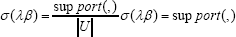 ; Where dentes the cardinality of U, and U represents the full universe of objects in decision table A.
Accuracy (or certainty factor): Accuracy is associated with every decision rule and is denoted accuracy ( λ β) or cer ( λ β. The accuracy is an indicator of how trustworthy a rule is in making a decision p given the condition λ. It is a frequency-based estimate of the conditional probability Pr ( β | λ), and is defined
as: accuracy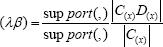 ; where C(x) represent a
pattern for condition attributes support represents a pattern in decision attribute. Accuracy or certainty factor is also called a confidence coefficient. A certainty factor of 1 represents a certain decision rule, and if 0<cer ( λ β)<1 the decision rule is called uncertain decision rule. In the context of lower and upper approximation sets, certain decision rules correspond to the lower approximation sets whereas uncertain decision rules correspond to the boundary region [18].
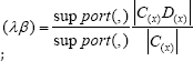
Coverage: The coverage of a decision rule is denoted coverage (λ β). The coverage gives a measure of howgood the pattern À describes the decision class defined by β. The coverage is also a frequency-based estimate of the conditional probability Pr (λ β), and is defined as: coverage
Setup of BMP economic costs for rough set application
Discretization of BMP economic costs data: The eleven (11) year BMP economic costs data is converted into a unit interval from zero (i.e. 0.00) to one (i.e. 1.00) using the re-scaling
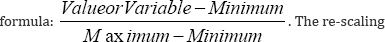
does not change the distribution of the original yield data, and the original values can be obtained by applying the inverse of the re-scaling factor. To apply rough sets to temporally varying economic costs data, the unit interval is discretized into set categories for analysis. Discretization may be based on equal frequency binning, entropy algorithm, manual discretization, and naïve or semi-naïve algorithms. In this paper, manual discretization is used and it is based on descriptive statistics for the BMP economic costs data. Based on the descriptive statistics the economic costs data is discretized into the following intervals.
Category 1: very low (VL)....................0.00 - 0.10
Category 2: low (L) 0.11.................... 0.20
Category 3: medium low (ML)..................0.21 - 0.40
Category 4: medium high (MH).................0.41 - 0.60
Category 6: very high (VH)....................0.81 - 1.00
Reduct approximation: The economic cost data from the first year (i.e., 1995) to the last year (i.e., 2005) are used as attributes. Since all the attributes are indicators for economic cost, the pattern for each sub-basin and subsequent reduct approximation are based on cardinality. For example, if the pattern for a subbasin is: High cost (8), Medium cost (2), and Low (1); that is, the sub-basin has a cardinality of 8 for high costs, 2 for medium cost, and 1 for low cost. The pattern definition does not consider if all the 8 high cost occurred sequentially or are interrupted by other cost groups. In other words, the sequence of attribute values is not considered in the indiscernibility relation between pairs of sub-basins. Suppose a pair of sub-basins (X and Y) has the same cardinality for X and Y which is described as Low cost (7), High cost (1), and Medium cost (3). The basis of discerning between the pair of sub-basins (X and Y) is not whether X and Y have the same sequence of economic cost. Rather, the pair (X and Y) is not discernible since their cardinalities are similar
Based on the subgroup definition for economic cost, the minimum number of attributes which can be used to approximate the same classification as the whole set of attributes is set to five (5). Specifically, a five year economic cost data will give a similar economic cost for a sub-basin as an eleven year economic cost data. This reduct approximation is based on the economic cost data for the three BMPs and therefore applies to the three BMPs: filter strip, zero tillage, and crop rotation.
Approximation of lower and upper sets: Lower and upper approximation sets are determined based on reduct approximation and cardinality (i.e., the number of instances a sub-catchment is associated with a particular economic cost category). Set criteria for the approximation of lower and upper approximation sets are defined in Table 7.

Upper approximation set: a sub-basin is a member of an upper approximation set for a particular cost category if its cardinality is 5 and above. Since reduct approximation is 5, a subbasin which has a cardinality of 5 for a specified cost category qualifies to belong to the specified cost category
Lower approximation set: since members of the lower approximation set must show a persistent membership to a particular cost category in order to qualify as definite members, the cardinality is fixed at 8 and above. Specifically, a sub-basin is a member of a lower approximation set for a particular cost category if its cardinality to the cost category is between 8 and11.
Boundary region: are sub-basins which belong to the upper approximation set but are excluded from the lower approximation set. Therefore, a sub-basin is placed into a boundary region for a particular cost category if its cardinality is between 5 and 7.
The definitions for upper approximation set and the boundary boundary region in order to restrict sub-basins to a single cost region creates the possibility for sub-basins to belong to two category. boundary regions of different costs categories. For example, a sub-basin may have a cardinality of 5 for one cost category and a cardinality of 6 for another cost category. Based on the definition of the boundary region, such a sub-basin qualifies to belong to both boundary regions for the two different cost categories. As a result, the following criterion is added to the definition for the boundary region in order to restrict sub-basins to a single cost category.
Boundary region: if a sub-basin belong to two boundary regions for different cost categories, then find the average of the constituent attributes values and put the sub-basin into the boundary region of the cost category into which the average valu falls,


Notes: the superscripts L and B denote a lower approximation set and
It is worth noting that the set criteria definition can vary based on the number of attributes (or years) so the set criteria is not rigid but can be modified to reflect different numbers of attributes. The set approximation criteria are exhaustive for the number of attributes and the set intervals evaluated. The use of rough sets is not limited to rigid number of set categories and intervals as illustrated in Table 7, but the number of set categories can be varied and the intervals may be defined based on skewed or non-skewed distribution.
Results and Discussion
Applying rough sets method to historical economic costs data
The information in Table 8 shows a sample collection of sub-basins and their corresponding economic costs for conservation tillage from 1995 to 2005. The corresponding patterns and the numerical measures generated from the sample sub-basins are shown in Table 9.
From Table 8, each sub-catchment has economic costs belonging to different economic cost categories. Apparently, individual sub-catchments do not belong to a consistent economic costs category. As a result, the sub-catchments are un- definable by their corresponding economic costs, and they have multiple economic cost memberships. In Table 9, the pattern for sub-basin 28 is L 4); ML(7), which indicates that the sub-basin 28 has a cardinality of 4 for low economic costs and a cardinality of 7 for medium low economic costs. Applying the rough sets approximation criteria, the sub-basin 28 is placed into the boundary region of medium low economic costs denoted MLB. From the information in Table 9, sub-basin 28 has a support value of 2 since there are two sub-basins (1 and 28) which have the pattern's antecedent, L (4); ML (7) and the pattern's consequent, ML. The remainder ofthe numerical measures for sub-basin 28 are
The above computation is repeated for the other sub-basins and the resulting values are shown in Table 9. In sum, economic costs for sub-basins are analyzed based upon their individual cost distribution at an instant. Numerical accuracy measures are also generated to evaluate the rough sets approximation. For example, support describes the frequency of a pattern, and coverage evaluates the consistency between a pattern and its corresponding decision. As a result, the approach can identify patterns which are more consistent as well as patterns which are uncertain. In other words, some economic costs categories are more variable than others. For example, the pattern for subbasin 48 is quite stable as its coverage and certainty values are both 1. But it worth noting that the pattern for sub-basin 48 is not common as its support is only 1 and its decision attribute is unique in Table 9. The rough sets approximation is applied to the economic costs data for the three BMPs, conservation tillage, filter strips, and crop rotation.
Rough sets decision for economic costs of BMPs
The rough set estimate of economic costs of BMPs is presented in Figure 4. The high levels economic costs are found at locations in the middle of the watershed, with the low levels clustered around upstream and downstream locations of the watershed. The medium low costs is uniformly spread throughout the entire watershed. The rough set costs represent the spatiotemporal distribution of BMP costs that are persistent temporally over the 11 year period. For BMP placement, this pattern of economic costs is expected to remain the same over several years

The estimated roughtset cost isevaluated byusing two evaluation measures: coverage and strength. The spatial distributions of the pattern of coverage and strength are shown in Figure 5. That is, for each sub-basin the estimated rough set cost can be examined in relation to its associated coverage and strength. The coverage measures the consistency of the rough set pattern; it indicates the roughness of the decision table. The coverage output shows that the coverage for a majority of sub- basins is between 3% and 12%. The minimum coverage is greater than 0%, all sub-basins have been successfully categorized into an economic cost group.

The strength indicates the relative occurrence of a rough set pattern for each sub-basin. The strength output shows that the strength for a majority of sub-basins is between 1% and 3%. The minimum coverage is greater than 0%, meaning that for any given sub-basin there are corresponding sub-basins with the same rough set pattern. Practically, this is crucial information in terms of BMP placement, because it means that there are options in terms of location or sub-basin which have same pattern of economic costs [29-32].
Validation of rough sets decisions
The estimated rough set cost is further evaluated by comparing its values against the economic costs for 2004 and 2005, in Figure 6 and Figure 7 respectively. For both 2004 and 2005 evaluations, the spatial distributions of economic costs in 2004 and 2005 against the rough set estimate is very similar. The similarity indexes for 2004 and 2005 are about 82% and 80% respectively. The high similarity further validates the rough set procedure in its estimation of economic costs of BMPs.


Conclusion
This study has provided a new methodology to estimate the economic costs of BMPs. The method is based on rough sets, and has a unique property of accounting for spatiotemporal variations of input variables used in determining the economic costs of BMPs. The rough sets method of determining economic costs of BMPs has been developed and demonstrated in this study for an agricultural watershed in southern Ontario, Canada. The BMPs examined include conservation tillage, crop rotation and filter strip for eleven year period between 1995 and 2005 inclusive.
The resulting rough set output includes an estimate of the economic costs of BMPs together with evaluation measures of support, strength, accuracy and coverage. The evaluation measures provide crucial information to examine the estimated BMP cost. The coverage output provides a level of flexibility for BMP placement by identifying optional locations or sub-basins with the same rough set pattern. Consequently, the rough set output is of direct significance to BMP placement and at optimal cost.
The rough set output was further validated by comparing its estimate of BMP cost to known BMP costs in 2004 and 2005. The comparison showed high level of similarity or about 80%, between the rough set estimate and the known values in 2004 and 2005. Together, these findings illustrate the rough sets approach as a highly capable method to robustly determine the economic costs of BMPs. The rough sets approach is advantageous in terms of its ability to determine patterns that are persistent across time periods. The flexibility of the rough set procedure to approximate cost categories for both limited and extended time periods makes it applicable for use with practical data sets.
References
- Dai C, Cai YP, Ren W, Xie YF, Guo HC (2016) Identification of optimal placements of best management practices through an interval-fuzzy possibilistic programming model. Agricultural Water Management 165: 108-121.
- Humenik FJ, Smolen MD, Dressing SA (1987) Pollution from nonpoint sources: where we are and where we should go. Environmental Science and Technology 21(8): 737-742.
- Stewart BA (1987) The U.S.D.A. Agricultural Research Service Commitement to Ground Water Research. In Ground Water Quality and Agricultural Practices, edited by D. M. Fairchild. Chelsea, Lewis Publishers Inc., Michigan, USA, pp. 1-5.
- DeBoe Gwendolen, Stephenson K (2016) Transactions costs of expanding nutrient trading to agricultural working lands: A Virginia case study. Ecological Economics 130: 176-185.
- Agriculture and Agri-Food Canada (2005) The National Environmental Farm Planning Initiative. Toronto, USA.
- Archer DW, Pikul JL, Riedell WE (2002) Economic risk, returns and input use under ridge and conventional tillage in the northern Corn Belt, USA. Soil and Tillage Research 67: 1-8.
- Epplin FM, Stock CJ, Kletke DD, Peeper TF (2005) Economies of size for conventional and no-till wheat production. Southern Agricultural Economics Association Annual Meeting.
- Kelly TC, Lu YC, Teasdale J (1996) Economic-environmental tradeoffs among alternative crop rotations. Agriculture, Ecosystems and Environment 60(1): 17-28.
- Kirwan B, Lubowski RN, Roberts MJ (2005) How cost-effective are land retirement auctions? Estimating the difference between payments and willingness to accept in the conservation reserve program. American Journal of Agricultural Economics 87: 1239-1247.
- Nakao M, Sohngen B, Brown L, Leeds R (1999) The Economics of Vegetative Filter Strips.OSU Extension.
- Anbumozhi V, Yamaji E (2001) Riparian land use and management of nonpoint source pollution in a rural watershed. Journal of Rural Planning Association 20: 55-59.?
- Lintner AM, Weersink A (1999) Endogenous Transport Coefficients. Environmental and Resource Economics 14: 269-296.
- Muleta MK, Nicklow JW (2002) Evolutionary algorithms for multiobjective evaluation of watershed management decisions. Journal of Hydroinformatics 4(2): 83-97.
- Yang W, Khanna M, Farnsworth R, Onal H (2003) Integrating economic, environmental and GIS modeling to target cost effective land retirement in multiple watersheds. Ecological Economics 46: 249-267.
- Dumedah G, Walker J, Chik L (2014) Assessing artificial neural networks and statistical methods for infilling missing soil moisture records. Journal of Hydrology.
- Dumedah G, Schuurman N, Yang W (2008) Minimizing effects of scale distortion for spatially grouped census data using rough sets. Journal of Geographical Systems 10(1): 47-69.
- Ohrn A (1999) Discernibility and Rough Sets in Medicine: Tools and Applications, Computer and Information Science. Norwegian University of Science and Technology, Trondheim.
- Pawlak Z (1982) Rough sets. International Journal of Computer and Information Sciences 11: 341-356.
- Yiridoe EK, Weersink A, Hooker DC, Vyn TJ, Swanton C (2000) Income Risk Analysis of Alternative Tillage Systems for Corn and Soybean Production on Clay Soils. Canadian Journal of Agricultural Economics 48(2): 161-174.
- Yang W, Isik M (2004) Integrating Farmer Decision Making to Target Land Retirement Programs. Agricultural and Resource Economics Review 33(3): 233-244.
- OMAFRA (2002) Soil Management and Fertilizer Use: Crop Rotation. Ontario Ministry of Agriculture Food and Rural Affairs, Canada.This work is licensed under Creative Commons Attribution 4.0 License DOI: 10.19080/ARTOAJ.2017.10.555785
- AGRICORP Canada (2006) Field crop yields: 1995 - 2005.
- OMAFRA (2002) Field Crop Statistics. Guelph: Ontario Ministry of Agriculture Food and Rural Affairs, Canada.
- OMAFRA (2007) Agronomy Guide for Field Crops. Publication 811 Ontario Ministry of Agriculture Food and Rural Affairs 2002.
- Uri ND (2000) The economic benefits and costs of conservation tillage. Environmental Geology 39(3-4): 238-248.
- Pawlak Z, Grzymala-Bausse J, Slowinski R, Ziarko W (1995) Rough sets. Emerging Technologies; Communication of the ACM 38 (11): 89-95.
- Pawlak Z (1997) Rough set approach to knowledge-based decision support. European Journal of Operational Research 99: 48-57.
- Zhang J, Goodchild MF (2002) Uncertainty in Geographical Information. Taylor & Francis, New York, USA.
- Choi SW, Sohngen B (2003) The optimal choice of residue management, crop rotations, and the cost of soil carbon sequestration. Canada.
- Duda AM (1993) Addressing nonpoint sources of water pollution must become an international priority. Water Science & Technology 28(3-5): 1-11.
- Dumedah G, Schuurman N (2008) Minimizing the effects of inaccurate sediment description in borehole data using rough set theory and transition probability. Journal of Geographical Systems 10(3): 291-315.
- Koo SM, Williams JR, Schurle BW, Langemeier MR (2000) Environmental and economic tradeoffs of alternative cropping systems. Journal of Sustainable Agriculture 15: 35-58.


