Review Article

Application of (bio)chemical engineering concepts and tools to model GRCs, and some essential CCM pathways in living cells. Part 2. Mathematical modelling framework

Gheorghe Maria*

Department of Chemical and Biochemical Engineering, Politehnica University of Bucharest and Romanian Academy, Chemical Sciences section, Romania

Submission: December 05, 2023; Published: January 25, 2024

*Corresponding author: Gheorghe Maria, Department of Chemical and Biochemical Engineering, Politehnica University of Bucharest, and Romanian Academy, Chemical Sciences section, Romania

How to cite this article: Gheorghe Maria*. Application of (bio)chemical engineering concepts and tools to model GRCs, and some essential CCM pathways in living cells. Part 2. Mathematical modelling framework. Ann Rev Resear. 2024; 10(3): 555790. DOI: 10.19080/ARR.2024.10.555790

Abstract

As proved by the recent literature, the developed in-silico (math-model-based) numerical analysis of such biochemical/biological systems turned out to be a beneficial tool to (i) off-line determine optimal operating policies of complex multi-enzymatic or biological reactors with a higher precision and predictability, or (ii) to design GMO (genetically modified micro-organisms) of desired characteristics for various uses. This work presents a holistic ‘closed loop’ approach that facilitate the control of the in vitro through the in-silico development of dynamic models for living cell systems, by deriving deterministic modular structured cell kinetic models (MSDKM) (with continuous variables and based on cellular metabolic reaction mechanisms). The ever-increasing availability of experimental (qualitative and quantitative) information about the tremendous complexity of cell metabolic processes, stored in large bio-omics databanks (including genomic, proteomic, metabolomic, fluxomic cell data for various micro-organisms), but also about the bioreactors’ operation necessitates the advancement of a systematic methodology to organise and utilise these data. This work is aiming to prove the feasibility and the advantages of using the classical and novel concepts and numerical tools of the chemical and biochemical engineering (CBE) to develop MSDKM of the extended cell-scale CCM-based (central carbon metabolism), and of genetic regulatory circuits (GRC) / networks (GRN). These extended kinetic models will be further linked to those of the bioreactor dynamic models (including macro-scale state variables), thus resulting hybrid structured modular dynamic (kinetic) models (HSMDM) proved to successfully solve more accurately difficult bioengineering problems compared to the classic (default) unstructured (apparent) math dynamic models. In the HSMDM, the cell-scale model part (including nano-level state variables) is linked to the biological reactor macro-scale state variables for improving both model prediction quality and its validity range.

By contrast, as proved in the 3&4 parts of this work, by considering only the macroscopic key-variables of the process (biomass, substrate, and product concentrations), and ignoring detailed representations of metabolic cellular processes, the unstructured (apparent, global) math dynamic models do not adequately reflect the metabolic changes of the bioreactor biomass, being inadequate to accurately predict the cellular response to the medium disturbances through the self-regulated cellular metabolism. These classical global/unstructured dynamic models may be satisfactory for an approximate modeling of the biological process, but not for modeling of cellular metabolic processes, and they cannot make any correlation between the bioreactor operation and the continuous adaptation of the biomass metabolism to the variable conditions of the bioreactor. Even worse, as proved by the author in previous papers, such global models may lead to biased and distorted conclusions about the GERM’s performances, thus making the modular constructions of GRC-s difficult by linking individual GERM-s.

In this 2nd part of the paper, a special attention is paid to the conceptual and numerical rules used to construct various individual GERM-s kinetic models, but also various GRC-s (e.g. toggle-switch, amplitude filters, modified operons, etc.) modular kinetic models from linking individual GERM-s. To develop more accurate and realistic math (kinetic) models of GERM-s and GRC-s, this part briefly reviews sa novel holistic ’whole-cell of variable-volume’ (WCVV) modelling framework introduced and promoted by the author in previous works. The WCVV has been proved to be more realistic and robust, by explicitly including in the MSDKM math-model relationships linking the cell-volume growth with the species dynamic mass balances, with also preserving the cell-osmotic pressure (that is the cell membrane integrity). The added isotonicity constraints were proved to be essential for more adequately predicting the performance regulatory indices (P.I.) of GERM-s and GRC-s. More specifically, this part briefly reviews the WCVV deterministic model hypotheses, and its advantages when simulating GERM-s, and GRC-s dynamics in living cells, by contrast to the classical (default) WCCV (whole-cell constant-volume modelling framework); regulatory performances indices (P.I.-s) of GERM-s; rules to link GERM-s when modelling GRC-s, and other related theoretical aspects.

Keywords: Biochemical engineering concepts applied in bioinformatics; Deterministic modular structured cell kinetic model (MSDKM); Hybrid structured modular dynamic (kinetic) models (HSMDM); Whole cell variable cell volume (WCVV) modelling framework; Whole cell constant cell volume (WCCV) modelling framework; Individual gene expression regulatory module (GERM); Genetic regulatory circuits (GRC), or networks (GRN); GERM regulatory performances indices (P.I.-s); Chemical and biochemical engineering principles (CBE); Rules of the control theory of nonlinear systems (NSCT); Whole-cell dynamic math models (WC); Gene circuit engineering (GCE)

Abbreviations: ADP: Adenosine-Diphosphate; AMP: Adenosine-Monophosphate; ATP: Adenosine-Triphosphate; BCE: (Bio)Chemical Engineering; CBE: Chemical and Biochemical Engineering; BR: Batch Reactor; CABEQ J: Chemical and Biochemical Engineering Journal; CCM: Central Carbon Metabolism; CIT: Citrate; CSTR: Continuous Stirred Tank Reactor; FBA: Flux Balance Analysis; FBR: Fed-Batch Bioreactor; G: The Active Gene (DNA); GCE: Gene Circuit Engineering; GERM: Individual Gene Expression Regulatory Module; GMO: Genetically Modified Micro-Organisms; GP: The Inactive Complex of G with the Transcription Factor P (its Encoding Protein in the Reduced Model here); GRC: Genetic Regulatory Circuits; GRN: Genetic Regulatory Networks; GS: Genetic Switch; HSMDM: Hybrid Structured Modular Dynamic (Kinetic) Models; L: Species at which Regulatory Element Acts; M: MRNA; MCA: Metabolic Control analysis; Met (MetG, MetP): Metabolites (Lumped DNA and Protein Precursor Metabolites, respectively); MINLP: Mixed-Integer Nonlinear Programming; MSDKM: Deterministic Modular Structured Cell Kinetic Model; MFA: Metabolic Flux Analysis; NLP: (Non)Linear Programming Problem [131]; NM: Nano-Moles/L, Nano-Molar (i.e. 10-9 Mol/L Concentration); NG: Negligible; NSCT: The Control Theory of Nonlinear Systems; Nut (NutG, NutP): Nutrient (External Nutrients Imported to Produce Metabolites Involved in the G and P Synthesis respectively); ODE: Ordinary Differential Equations Set; P: Protein; P.I.-s: GERM Regulatory Performances Indices; PTS: Phosphotransferase GLC Import System; PPP: Pentose-Phosphate Pathway; SCR: Semi-Continuous Bioreactor; SNP: Single Nucleotide Polymorphisms; SUCC: Succinate; Re(x): Real part of ”x” Variable; TF: Transcription Factor; TCA: Citric Acid Cycle (or Tricarboxylic Acid Cycle); TPFB: Three-Phase Fluidized Bioreactor; TRP: Tryptophan; QSS : Quasi Steady-State; WC: Whole Cell; WCCV: Whole Cell of Constant Volume Hypothesis; WCVV: Whole Cell of Variable Volume Hypothesis; [.]: Concentration

Part 1: (General concepts) of this work is published with Current Trends in Biomedical Eng & Biosci., (Juniper, Irvine CA, USA), 22(1), 556080-556104 (2023), ISSN: 2572-1151, DOI: 10.19080/CTBEB.2023.22.556080

Part 2: (Mathematical modelling framework) of this work is the present paper.

Part 3: (Applications in the bioengineering area) of this work is in-press with Archives in Biomedical Engineering & Biotechnology, (Iris publ, San Francisco CA, USA), 2024, ISSN: 2687-8100, ABEB MS.ID.000672. DOI: 10.33552/ABEB.2024.07.000672.

Part 4: (Applications in design some GMO-s) of this work is published with Annals of Systems Biology, (Peertechz publ, Los Angeles, USA), ISSN: 2692-4765, vol. 7(1), pp. 001-034, January 19 - 2024, Article ID: ASB-7-121, https://doi.org/10.17352/asb.000021

Introduction

As discussed in the Part-1 of this work, the current off-line insilico approach (based on the math models) used in biochemical engineering and bioengineering practice for solving desisgn, optimization and control problems of industrial biological reactors is to use unstructured Monod (for cell culture reactor) or Michaelis-Menten (if only enzymatic reactions are retained) by ignoring detailed representations of metabolic cellular processes, or interactions among enzymatic reactions in multi-enzymatic systems. As discussed, the applied engineering rules are imported or are like those used in the chemical and biochemical engineering (CBE), and in the control theory of nonlinear systems (NSCT), and Bioinformatics. However, by considering only the macroscopic key-variables of the process (biomass, substrate, and product concentrations), these unstructured (apparent, global) math models do not adequately reflect the metabolic changes of the bioreactor biomass, being inadequate to accurately predict the cellular response to the medium disturbances through the selfregulated cellular metabolism over dozens of cell cycles. These global dynamic models may be satisfactory for an approximate modeling of the biological process, but not for modeling of cellular metabolic processes, and they cannot make any correlation between bioreactor operation and the continuous adaptation of biomass metabolism to the variable conditions of the bioreactor. Even worst, as proved by [1-9], such global CCM models, or the whole-cell (WC) math kinetic models of GERM-s (individual gene expression regulatory modules), or for GRC-s (genetic regulatory circuits) constructed in a WC constant cell volume (WCCV) modelling framework, may lead to biased and distorted conclusions about the GERM’s performances, thus making difficult the modular constructions of GRC-s by linking individual GERM-s [1,2,4-9].

The current trend to solve such engineering problems more accurately is to use deterministic modular structured cell kinetic models (MSDKM), or hybrid structured modular dynamic (kinetic) models (HSMDM) with continuous variables, and based on cellular metabolic reaction mechanisms, that consider, with a degree of detail suitable to the each approached case study, the cellular metabolic reactions and the cell key-species dynamics. In the HSMDM, the cell-scale model part (including nano-level state variables) is linked to the biological reactor macro-scale state variables for improving both model prediction quality and its validity range. As proved ny Maria [1-5], and Yang et al. [10], the modular structured kinetic models can reproduce the dynamics of complex metabolic syntheses inside living cells. This is why the modular GRC dynamic models, of an adequate mathematical representation, seem to be the most comprehensive mean for a rational design of the regulatory GRC with desired behaviour [11]. These structured dynamic math models (MSDKM, or HSMDM) can satisfactorily represent the key steps of the central carbon metabolism (CCM) at a cell scale, by also including reaction modules responsible for the synthesis of cellular metabolites of interest for the industrial biosynthesis. The same MSDKM can satisfactorily simulate, on a deterministic basis, the self-regulation of cell metabolism for its rapid adaptation to the changing bioreactor reaction environment, by means of complex “genetic regulatory circuits” (GRC-s), which include chains of individual „gene expression regulatory modules” (GERM-s).

In this way, more accurate predictions are obtained both for the dynamics of the biological process at the cellular level, and for the dynamics of the operating parameters of the analyzed industrial bioreactor. The immediate applications of these MSDKM and HSMDM refer to (i) the more precise determination of the optimal operating policy of an industrial bioreactor, and (ii) facilitates, by means of an in-silico (math-model based) numerical analysis, determination of GMO-s with a cell metabolism of desired characteristics [12-16]. In this context, this 2nd part of the work shortly review the essential CBE and NSCT principles and rules used to elaborate MSDKM, but also the so-called „Hybrid structured modular dynamic (kinetic) models” (HSMDM) with continuous variables [12,13,15] that combine the characteristics of the cellular metabolic process involving species participating to the essential reaction modules of CCM (Figure 1 & Figure 2) at a nano-scopic level, with the macro-scopic processes involving the state variables of the industrial bioreactor. Special attention is paid to the conceptual and numerical rules used to build-up modular CCM kinetic models, in direct connection to various individual GERM-s kinetic models, but also to various GRC-s (e.g. toggle-switch, amplitude filters, operons expression, etc.) modular kinetic models by linking a couple of GERM-s. To do such a complex modelling work in a consistent way, this 2nd part of the work will briefly reviews the novel „Whole cell variable cell volume” (WCVV) modelling framework introduced and promoted by the author in previous works, such as [1,2,4-6,8,9,17], as an essential modelling instrument to develop more realistic and precise MSDKM-s and HSMDM-s. Besides presenting the WCVV deterministic model hypotheses, this paper points-out its advantages when simulating GERM-s, and GRC-s dynamics in living cells, in a holistic approach, by contrast to the classical (default) WCCV (whole-cell constantvolume modelling framework). Even worst, as proved by [1,2,4- 6,8,9], such global CCM models, or the whole-cell (WC) math kinetic models of GERM-s, or for the GRC-s constructed in a WC constant cell volume (WCCV) modelling framework, may lead to biased and distorted conclusions about the GERM’s performances, thus making difficult the modular constructions of GRC-s by linking individual GERM-s.

The novel WCVV has been proved to be more realistic and robust [1,2,4-6,8,9], by explicitly including in the MSDKM mathmodel relationships linking the cell-volume growth with the species dynamic mass balances, with also preserving the cellosmotic pressure (that is the cell membrane integrity). The added isotonicity constraints were proved to be essential for more adequately predicting the performance regulatory indices (P.I.) of GERM-s and GRC-s. More specifically, this part briefly reviews the WCVV deterministic model hypotheses, and its advantages when simulating GERM-s, and GRC-s dynamics in living cells, by contrast to the classical (default) WCCV ; regulatory performances indices (P.I.-s) of GERM-s; rules to link GERM-s when modelling various GRC-s (e.g. toggle-switch, amplitude filters, modified operons, etc.), and other related theoretical aspects. As is proved in the Parts 3 and 4 of this work, the in-silico (math/kinetic modelbased) numerical analysis of biochemical or biological processes by using MSDKM or HSMDM models are proved to be not only an essential but also an extremely beneficial tool for engineering evaluations aiming (i) to determine with a higher accuracy the optimal operating policies of complex multi-enzymatic reactors, [18-23], or of bioreactors including the biomass adaptation to the variable bioreactor environment over hundreds of cell cycles [12- 14, 24-27], or even (ii) to easier and quickly simulate and analyze the performances/ characteristics of various GMO-s alternatives, by using the “metabolic flux analysis” (MFA) [27-31], together with the gene-knock-out technique, or the cell cloning procedure [4,5,12-15,31,32].

A central part of cell metabolic math (kinetic) models concerns self-regulation of the metabolic processes via GRC-s. Consequently, one application of such dynamic cell MSDKM or HSMDM models is the study of GRC-s, connected to the CCM reaction modules to predict ways by which biological systems respond to signals, or environmental perturbations. The emergent field of such efforts is the so-called ‘gene circuit engineering’ (GCE), that is a part of the Synthetic Biology (see the Part-1 of this work), and many examples have been reported with in-silico re-creation of GRC-s conferring new properties/functions to the mutant cells. Thus, Synthetic Biology was defined as “putting engineering into biology”. [33]. This emerging field is strongly linked to the Systems Biology which, is one of the modern tools, that uses advanced mathematical simulation models for in-silico design of GMOs that possess specific and desired functions and characteristics. By using simulation of gene expression, the GCE realizes in-silico design of GMO-s that possess desired cell functions. By inserting new genes or knock-out some of them, modified GRC-s can be obtained inside a target micro-organism, thus creating a large variety of mini-functions / tasks (desired ‘motifs’) to the mutant (GMO) cells in response to external stimuli [4,5,32-39,40-48]. This needs to have good quality MSDKM structured cell models to simulate the dynamics of the bacteria CCM (and its regulation via cell GRC-s/GRN-s) became a subject of very high interest over the last decades, allowing in-silico design of GMO-s with desirable characteristics of various applications in the biosynthesis industry, civil engineering, medicine, and other fields [1,2,4,5]. This important motivation fully justifies derivation of more accurate and realistic modelling frameworks of CCM and GERM-c / GRC-s, as those described in the next section.

2. Modelling the Dynamics of GRC/GRN in Living Cells

Because the GRC-s are responsible for the control of the cell metabolism, the adequate kinetic modelling of the constitutive GERM-s, but also the adequate representation of the linked GERM regulatory efficiency in a GRC is an essential step in describing the cell metabolism regulation via the hierarchically organized GRC-s (where key-proteins play the role of regulatory nodes). Eventually, such models allow simulating the metabolism of modified cells [1,2,4,5]. Various reduced / extended math (kinetic) models have been proposed to represent the elementary metabolic fluxes of a CCM (Figure 1 & Figure 2). (see the reviews of [49,48,1,2,4,5]), or of various GRC-s [12-14, 35-39, 50-73, 1,2,4,5]. Eventually, such models allow a multi-criterion design and optimization of a target GRC-s [12-14,74]. Generally, living cells are evolutionary, autocatalytic, self-adjustable structures able to convert raw materials from the environment into additional copies of themselves. Living cells are hierarchically organized, self-replicating, evolvable, and responsive biological systems to environmental stimuli. The structural and functional cell organization, including components and reactions, is extremely complex, involving O (103- 4) components, O (103-4) transcription factors (TF-s), activators, inhibitors, and at least one order of magnitude higher number of (bio)chemical reactions, all ensuring a fast adaptation of the cell to the changing environment [1,2,4,5, 73-76]. Relationships between structure, function and regulation in complex cellular networks are better understood at a low (component) level rather than at the highest-level [77,78].

Cell regulatory and adaptive properties are based on homeostatic mechanisms, which maintain quasi-constant keyspecies concentrations and output levels (i.e. quasi-steady-state - QSS, of a cell balanced growth) by adjusting the synthesis rates, by switching between alternative substrates, or development pathways. Cell regulatory mechanisms include allosteric enzymatic interactions and feedback in gene transcription networks, metabolic pathways, signal transduction and other species interactions [79]. Protein synthesis homeostatic regulation includes a multi-cascade control of the gene expression with negative feedback loops and allosteric adjustment of the enzymatic activity [1,2,4,5,73,75,76,80,81]. When the cell-model used to construct an extended HSMDM includes individual GERM-s of various types (Figure 3 & 4) [1,2,4,5,73], or complex GRC-s gathering chains of inter-connected GERM-s, such as genetic switches (Figure 5), or operons’ expression (Figure 6), genetic amplifiers, etc. [1,2,4,5,57,75,82,83], the classical (default) is to use the ’whole-cell-constant-volume’ (WCCV) kinetic modelling, by writing the species differential mass balances in terms of concentrations but neglecting the cell-volume continuous growth. However, as proved by [1,6-9,17] this classic (WCCV) kinetic modelling framework cannot longer be applied because the regulatory properties of GERM / GRC are related to the cell holistic properties, in direct connection to the cell-volume growth, and to a lot of additional constraints derived from the cell holistic properties (e.g. isotonic constraint ensuring the cell membrane integrity).

To also account for the cell growth, and their holistic constraints, a novel holistic “whole-cell” (WC) math modelling framework of cell processes must be applied, to also account for the cell variable volume and other constraints. This novel WC math modelling framework was introduced by Maria [6,73,84], that is the so-called ’whole-cell-variable-volume’ (WCVV), by analogy with the CBE concepts/rules [85]. More specifically, WCVV uses the same concepts/principles and analytical/ numerical rules employed by CBE when developing kinetic models for chemical reactions conducted in variable-volume systems [85]. Implications of the novel WCVV concept when modelling metabolic cell processes (especially GRC-s) under variable cell-volume were systematically studied, compared to the WCCV models [6], positive results extrapolated, and widelly promoted in a large number of applications by Maria [1,2,4,5, 6-9, 12-15, 25,73,75,76,84,86-88] that is the so-called „whole-cellvariable- volume (WCVV) framework. The next chapters aim to briefly describe the characteristics of the WCVV approach, and its superiority in the prediction accuracy offered by the WCVV kinetic modelling framework compared to the classical WCCV, as proved by [1,2,4,5, 6-9,17].

In this context, the adequate modelling of the genetic regulatory circuits (GRC), made from linked GERM-s, together with modelling the cell central carbon metabolism (CCM) remain subjects of tremendous importance on which researches have been focus over the last decades, as long as GRC-s are the essential metabolic components used to re-design the whole cell metabolism, and in regulating the whole cell syntheses [1,73]. GRC-s, also denominated as ’genetic regulatory networks’ GRN-s, is a combination (network) of GERM-s ensuring precise functions into the cell (Figures 5 & 7). Due to the gene location in the GRC nodes, a more sophisticated definition was given by [89], by using the graph-theory:

Definition- Gene Regulatory Network (GRN): a Gene Regulatory Network is a mixed graph G: = (V, U, D) over a set V of nodes, corresponding to gene-activities, with unordered pairs U, the undirected edges, and ordered pairs D, the directed edges. A directed edge dij from vi to vj is present if a casual effect runs from node vi to vj and there exist no nodes or subsets of nodes in V that are intermediating the casual influence (it may be mediated by hidden variables, i.e. variables not in V). An undirected edge uij between nodes vi and vj is present if gene-activities vi and vj are associated by other means than a direct casual influence, and there exist no nodes or subsets of nodes in V that explain that association (it is caused by a variable hidden to V).

2.1. The modular modelling approach of GRC-s

In fact, any lumped representation of a GERM, or a GRC should include, in one form or another, the main ’actors’ of such regulatory circuits, that is: metabolites (Met*) as substrates for genes (MetG) and protein (MetP) synthesis, genes (G*) and their encoded proteins (P*), as depicted in (Figure 7). This is a very simplified representation of the biochemistry in living cells (“hiding” hundreds of enzymatic reactions) conceptually decomposed in three “spaces”. Influences between gene-activities, without explicitly accounting for the proteins and metabolites, result from a projection of all regulatory processes on the ‘gene space’ [90]. The used analysis of GRC-s/GRN-s is those of a modular one. Thus, more complex functions, such as regulatory networks, synthesis networks, or metabolic cycles can be built-up by using the building blocks rules [33]. The modular organization of cell regulatory systems is computationally very tractable. Moreover, it is known that one gene expression interacts with less than 23-25 other GERM-s [91], while most GERM structures are repeatable. Thus, to study one individual GERM, it is not necessary to model the whole cell GRN.

The modular GRC dynamic models, of an adequate math representation, seem to be the most comprehensive means for a rational design of the regulatory GRC-s with desired behaviour [11,73,76]. However, the lack of detailed information on reactions, rates and intermediates makes the extensive representation of the cell large-scale GRC–s difficult, if not impossible, for both deterministic and stochastic approach [41,73]. When continuous variable dynamic models are used, the default framework is that of a constant volume / osmotic pressure system (WCCV), by accounting for the cell-growing rate as a ‘decay’ rate of key-species (often lumped with the degrading rate) in a so-called ‘diluting’ rate. Such a representation might be satisfactory for many applications, but not for accurate modelling of cell regulatory / metabolic processes under perturbed conditions, or for division of cells, distorting the prediction quality [1,2,4,5, 6-9]. The variable-volume modelling framework WCVV detailed in this section, with explicitly linking the cell-volume growth, external conditions, osmotic pressure, cell content ballast (that is the cell content, expressed as a total concentration in nano-moles/cytosol volume), and net reaction rates for all cell-components, is proved as being more promising in predicting local and holistic properties of the CCM metabolic networks, or of various cell GRC-s [1,2,4,5,73,76], or even the cell cycle [92]. By contrast, the classical WCCV modelling framework tends to overestimate the GRC dynamic regulatory properties [6,7, 73,76,93,94].

2.2. Examples of such GRC modulated functions.

As mentioned by the pioneers of this field, with the aid of recombinant DNA technology, it has become possible to introduce specific changes in the cellular genome. This enables the directed improvement of certain properties of micro-organisms, such as the productivity in a target (excretable) metabolite, by changing the nature/amount of the encoded cell enzymes, which is referred to as Metabolic Engineering [2,4,5,28,95,96]. This is potentially a great improvement compared to earlier random mutagenesis experimental techniques but requires that the targets for modification are known. The complexity of pathway interaction and allosteric regulation limits the success of intuition-based approaches, which often only take an isolated part of the complete system into account. Mathematical models are required to evaluate the effects of changed enzyme levels or properties on the cell system taken as a whole (WC concept), by using the “metabolic control analysis” (MCA) or a dynamic sensitivity analysis [1,2,4,5,94,97]. In this context, GERM and GRC dynamic models are powerful tools in developing re-design strategies of modifying genome and gene expression seeking for new properties of the mutant cells in response to external stimuli [1,2,4,5]. Examples of such GRC modulated functions include toggle-switches, hysteretic GRC behaviour, GRC oscillator, specific treatment of external signals, GRC signalling circuits and cell-cell communicators [86]. Examples of such GRC modulated functions include [1,2,4,5,75,86,98]:

a) Toggle-switch, i.e. mutual repression control in two gene expression modules, and creation of decision-making branch points between on/off states according to the presence of certain inducers (Figure 5, with references).

b) Hysteretic GRC behavior, that is a bio-device able to behave in a history-dependent fashion, in accordance with the presence of a certain ‘inducer’ in the environment.

c) GRC oscillator produces regular fluctuations in network elements and reporter proteins and makes the GRC evolve among two or several quasi-steady states [48,99-103]. Complex MSDKM structured models including CCM and GRC modules can predict conditions for oscillations occurrence for various cell processes [36,48,82,99-101,149]. As studied by Yang et al. [149], “all biochemical reactions in organisms cannot occur simultaneously due to constraints of thermodynamic feasibility and resource availability, just as all trains in a country cannot run simultaneously. Therefore, oscillations provide overall planning and coordination for the inner workings of the cellular system. This seems to be contrary to the theoretical basis of GEMs, which are based on the steady-state hypothesis and flux balance analysis [104], but just as computers will not operate in the same way as the human brain, this difference can be understood and accepted, so that non-equilibrium theory and the steady-state hypothesis have been and will continue to coexist and guide our reasoning [149].

d) External signals treatment by controlled expression such as amplitude filters, noise filters or signal / stimuli amplifiers. For instance, the signal (external mercury) amplifier and quick induction of the mercury (MER)-operon expression in E. coli [5,13,14].

e) GRC signalling circuits and cell-cell communicators, acting as ‘programmable’ memory units, by adapting the cell metabolism to the environmental changes. See, for instance [4,5] for the mer-operon, and TRP-operon cases.

f) GRC for operon expression. For instance: mercury (MER)-operon expression in E. coli [5,13,14]; tryptophan (TRP)- operon expression [5,15].

As discussed by [1,2,4,5,6,17,73], the classical (default) modelling tools of metabolic cell processes are based on the ’Constant Volume Whole-Cell’ (WCCV) continuous variable ODE dynamic models which, do not explicitly consider the cell volume exponential increase during the cell growth. As proved by [6,8,9], such an approach may lead to biased and distorted conclusions on the GERM’s performances, thus making difficult the modular constructions of GRC-s by linking individual GERM-s. By contrast, the holistic ’whole-cell of variable-volume’ (WCVV) modelling framework introduced, extended, and widely promoted by [1,2,4,5,6-9, 13,14, 73,76,87,88] has been proved to be more realistic and robust, by explicitly including in the model relationships the cell-volume growth, with preserving the cellosmotic pressure (that is the cell membrane integrity). The added isotonicity constraint by Maria [1,2,4,5,6-9,73,84] proved to be essential for predicting more adequate performance regulatory indices (P.I.-s, see the below section) of GERM-s and GRC-s.

2.3. GRC comparative modelling using WCVV vs. WCCV

This section is aiming to exemplify, in a simple and meaningful way, the importance of using a WCVV modelling framework compared to the classical (default) WCCV models when simulating the main regulatory properties of GERM-s or GRC-s, by explicitly accounting for the cell-volume growth, and system thermodynamic isotonicity (constant osmotic pressure). Exemplification is made for the case of the simplest generic GERM model, of [G(P)1] type (see GERM nomenclature in the below sections and the subsequent references), with characteristics taken form E. coli cells [8,9, 73,75,105-107], by mimicking the cell homeostasis and its response to dynamic perturbations. The paper subject importance is very high, if many cell simulators are developed and used for practical applications in the biosynthesis industry, and in medicine. The isotonicity constraint is proving to be a natural way to preserve the homeostatic properties of the cell system [1,2,4,5,6,73,76], instead of imposing other constraints, such as “the total enzyme activity” and “total enzyme concentration” constraints [108,109]. A comparison of model prediction quality in the case of a GERM of [G(P)1] type (Figure 3 & Figure 4) modelled under WCCV or WCVV, clearly indicate that WCCV can lead to biased and distorted conclusions on GERM regulatory performances (under both stationary or as response to dynamic pulse-like perturbations), thus making difficult the modular construction of GRC-s by linking individual GERM-s (Figure 8 & Figure 9) [6,8,9].

2.3.1. WCCV modelling framework.

For a system of chemical or biochemical reactions conducted in a cellular defined volume ’V’ (assumed an open system of uniform content), the classical (default) formulation of the corresponding (bio)chemical kinetic models based on continuous variables (concentration vector ’C’, or number of moles vector ’n’) implies writing a set of ordinary differential equations (ODE) representing the mass balance of the considered system states (biological/chemical species index ’j’, taken individual or lumped), in the following WCCV (whole-cell constant-volume) modelling formulation (with referring to the whole system volume)[110]:

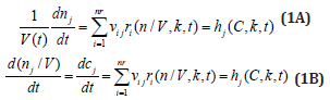
Where C_j = species “j” concentration; nj = species “j” number of moles; ν_ij = the stoichiometric coefficient of the species “j” in the reaction “i”; ri = reaction “i” rate. The above formulation assumes a homogeneous constant volume with no inner gradients or species diffusion resistance into the cell. When continuous variable ODE dynamic models are used to model cell enzymatic/metabolic processes, the default-modelling framework Eq. (1A-B) is that of a constant volume and, implicitly, of a constant osmotic pressure (π) in isothermal systems (to ensure the cell membrane integrity), according to the assumed fulfilled Pfeffer’s law in diluted solutions (i.e. the cytosol system) [73,84]:

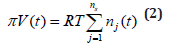
Where: T = absolute temperature, R = universal gas constant, V = cell (cytosol) volume; π = osmotic pressure; t = time; nj = species “j” number of moles. To overcome this drawback, some WCCV models accounts for the cell-growing rate as a pseudo- ‘decay’ rate of key-species (often lumped with the degrading rate) in a so-called ‘diluting’ rate denoted here by an average Ds [see below eq. (3B) and eq. (4A) for its significance). In fact, by ignoring the direct influence of the cell volume increase, the WCCV dynamic model cannot ensure the system isotonicity constraint fulfilment because the sum of species number of moles doubles over the cell cycle. Such a WCCV dynamic model might be satisfactory for modelling many cells sub-systems, but not for an accurate modelling of cell regulatory / metabolic processes under perturbed conditions, or for division of cells [92], distorting the prediction quality, as reviewed by [1,2,4-9,73]. Other researchers [109] tried to preserve the homeostatic properties of the cell system, not by imposing the isotonic constraint Eq. (2), but by means of “artificial” cell constraints, such as “the total enzyme activity” and “the total enzyme concentration” [108,109].

2.3.2. WCVV formulation

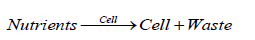
The WCVV (“whole cell variable cell volume”) modelling formulation is based on a couple of hypotheses, presented in this section. Life at its simplest level involves two major divisions of interacting molecular species called the cell and the environment. The environment consists of molecules dissolved in water and largely separated from the cell. In their simplest form, cells consist of hydrophilic molecules in aqueous volumes (cystosol), encapsulated by semi-permeable hydrophobic membranes composed of phospholipids and proteins [1,2,4-9,73]. Cellular components interact to catalyze the synthesis of more cells from environmental components called nutrients. Imported into the cell and transformed into metabolites. This auto-catalytic process is specified by the following overall auto-catalytic global lumped reaction:

As long as excess nutrients are available, this auto-catalysis causes cell populations to increase exponentially. The volume of a newborn cell doubles during its cell cycle. Cells contain nucleic acids (DNA, RNA, or both) and proteins, interrelated through the processes of transcription, translation and DNA replication. Taken together, these metabolic processes are mutually autocatalytic, as shown in the following overall schemes:

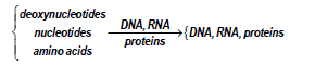
DNA and protein are co-catalysts for RNA synthesis from Ribonucleotides. In turn, RNA and proteins (enzymes) are co-catalysts for the synthesis of proteins from amino acids, of DNA (from the monomeric units called deoxyribonucleotides), RNA, and other proteins. The substrates for these processes (deoxyribonucleotides, nucleotides, amino acids etc.) are metabolites, synthesized from imported environmental nutrients through complex metabolic pathways [111]. “At this point, it is to strongly emphasize that living cells are systems of variable volume. They double their volume during the cell cycle. For chemical or biochemical systems of variable-volume, another formulation is more appropriate, being given by [86] for chemical reacting systems. Such CBE modelling tools were translated and promoted in developing structured math models of cell processes (that is CCM and GRC-s) by Maria [1,2,4-9, 73,75,76,84,87,93,112]. Such a novel kinetic modelling framework of cell systems by also including the cell isotonicity, and the variable cell-volume constraints in the so-called WCVV modelling framework (for details, see the last references from above). In mathematical terms, the species mass balance Eq. (1) should be re-written in the following form:

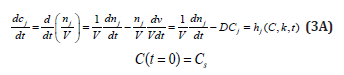
Where: C = cell species concentration vector; t = time; k = math model constants; ’s’ index = at steady-state; h = cell kinetic model functions. The variable “D” is the logarithmic growing rate of the cell volume, also known as the “cell dilution rate”, being defined by the following relationship:

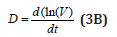
There are two possibilities to calculate the cell dilution ’D’ necessary for solving the model Eq. (3A). The simplest, but not the accurate one, is to use a value averaged over the whole cell cycle, that is:

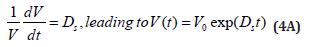
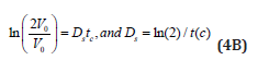
By accounting the cell double volume at the end of the cellcycle, then the constant Ds can be a-priori evaluated by using the following relationship (for cells of known cell cycle):

The second alternative, and the more rigorous way to evaluate the cell dilution ’D’ is to impose a constraint accounting for the cellvolume growth while preserving a constant osmotic pressure and membrane integrity. Thus, by derivation of the Pfeffer’s law Eq. (2) in respect to V, and by division to V, one obtains the ’isotonic’ dilution rate Di [1,6-9,73]:

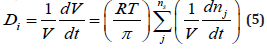
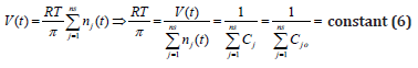
It is to observe in Eq. (5) that the cell content dilution rate Di is linked to the whole species (taken individually or lumped) reaction rates via the isotonicity constraint. As species reaction rates vary during the cell cycle, it clearly results that formulation Eq. (5) offers a more accurate estimation of the (variable) cell dilution at any time. Such a system isotonicity constraint is more ’natural’ and eventually includes” the total enzyme activity” and” total enzyme concentration” constraints suggested by [109]. In the above relationships eqns. (2, 5), the following notations have been used: T = absolute temperature, R = universal gas constant, V = cell (cytosol) volume. As revealed by Pfeffer’s law eqn. (2) in diluted solutions [113], and by the eq. (5), the volume dynamics is directly linked to the molecular species dynamics under isotonic and isothermal conditions. Consequently, the cell dilution ’D’ results as a sum of reacting rates of the all-cell species (individual or lumped). The (RT/π) term can be easily deducted in an isotonic cell system, from the fulfilment of the following invariance relationship derived from eqn. (2):

The basic hypotheses of the WCVV dynamic models of type Eqs. (3-6) are briefly presented in the (Table 1), and in the details below. These formulations are valid over ca. 80% of the cell cycle representing the balanced cell growth before its division [92]. The whole chemical/biochemical cell processes are called ’cell metabolism’, defined as: “Metabolism” is the set of life-sustaining chemical transformations within the cells of living organisms. The three main purposes of metabolism are the conversion of food/fuel to energy to run cellular processes, the conversion of food/fuel to building blocks for proteins, lipids, nucleic acids, and some carbohydrates, and the elimination of nitrogenous wastes. These enzyme-catalyzed reactions allow organisms to grow and reproduce, maintain their structures, and respond to their “environments” [111]. The basic equations and hypotheses of a deterministic WCVV simplified cell model (with continuous variables) presented in this work, also called a “mechanical cell”, are presented by [1,2,4-6,73], and summarized in (Table 1). To better underline the WCVV models hypotheses, a couple of issues should be explained, as followings [4,5]:

i) Genes (generically denoted by G), and the encoded proteins (generically denoted by P) are in a mutually auto-catalytic relationship: the synthesis of P is catalyzed by G, and vice-versa (directly or indirectly), in the so-called GERM-s (see the GERM library of (Figure 3).

ii) During its cell cycle, the cell is of variable volume, but preserving a constant osmotic pressure.

iii) The regulatory mechanisms to achieve the gene expression modelled by lumped GERM-s, and the internal homeostasis are explained in detail by [1,2,4-9,73] and shortly reviewed in the below sub-sections.

iv) The cell WCVV model assumes an ideal system, that is: isothermal and with a uniform content (perfectly mixed case); species behave ideally, and present uniform concentrations within cell. The cell system is not only homogeneous but also isotonic (constant osmotic pressure), with no inner gradients or species diffusion resistance.

v) The cell is an open system interacting with the environment through a semi-permeable membrane. To better reproduce the GERM properties interconnected with the rest of the cell, the other cell species are lumped together in the so-called” cell ballast” [1,2-9,73]. The cell-ballast has an important influence on the GERM performance indices (see below) through the common cell volume to which all species contribute.

vi) The inner osmotic pressure (πcyt) is constant, and all time equal with the environmental pressure, thus ensuring the membrane integrity (πcyt = πenv = constant [1,4]). Even if, in a real cell, such equality is approximately fulfilled due to perturbations and transport gradients, and despite migrating nutrients from environment into the cell, the overall environment concentration is considered to remain unchanged. On the other hand, species inside the cell transform the nutrients into metabolites and react to make more cell components. In turn, increased amounts of polymerases are then used to import increasing amounts of nutrients. The net result is an exponential increase of cellular components in time, which translates, through isotonic osmolarity assumption, into an exponential increase in volume with time [V = Vo exp(+Ds·t)] [see eqn. (3B,4A,4B,5)].

vii) Due to the “D” term in eq. (3A, 3B), the cell content reports a continuous dilution, that is a species concentration decline due to the continuous increase of the denominator of the expression Cj = nj(t)/V(t). Despite that, concentrations of key species remain constant because the numerator (copy numbers) increases at the same rate as the denominator. So, the overall concentration of cellular components is time-invariant at the cell homeostasis (i.e. quasi-steady-state, or balanced growth).

viii) Species concentrations at the cell level are usually expressed in nano-moles, being computed with the relationship of [73]:

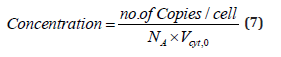
where NA is the Avogadro number. For instance, for an E. coli cell with an approximate volume of Vcyt,0 = 1.66 10-15 L [107], concentration of one generic gene G copynumber is: [G]s = (1/ (6.022×1023)(1.66×10-15) = 1 nM (that is 10-9 mol/L).

ix) Under quasi-stationary growing conditions (QSS), from eq. (1A, 3A) it results that species “j” synthesis rates (rj) must equal to first-order dilution rates (Ds Cj,s), leading to the timeinvariant (index ’s’) species concentrations Cj,s, i.e. the homeostatic conditions (corresponding to a balanced steady-state growth). Under QSS cell growing conditions, the ODE model mass balance eq. (3A) is leading to the following nonlinear algebraic mass balance set:

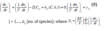
This QSS mass balance eq. (8) is used to estimate the rate constants ’k’ by using the known experimental stationary species concentration vector Cs, while also imposing some constraints to ensure the optimal properties of the cell system. Some examples are given by [1,2, 4-6,8,9,12-14,73,76,86,98,114].

x) It is to observe that, in a continuous variable cell kinetic model, species concentrations can present fractional values. When treated deterministically, fractional copy numbers must be loosely interpreted either as time-invariant average in a population of cells, or as a time-dependent average of single cells. For other types of cell kinetic models (with stochastic, or Boolean variables, topological, etc.) see the review of [1,2,4,5,73].

xi) A metabolic kinetic model in a WCVV approach should be written in the form eq. (3-6). In such a formulation, all cell species should be considered (individually or lumped), because all species net reaction rates contribute to the cell volume increase [see eq. (6)]. As the cell volume is doubling during the cell cycle, this continuous volume variation cannot be neglected.

The simplest representation of the core of such a ’mechanical cell’ is shown in (Figure 8-down-right). It exists in an environment consisting of two nutrients NutG and NutP. The cell contains one gene (lumped genome), and protein (lumped proteome) [12-14] in a mutually autocatalytic relationship, two lumped metabolites (METG and METP) used in the synthesis of the G/P pair, and various regulatory elements promoting internal homeostasis. A membrane is presumed to demarcate the cell from its environment but is not an explicit component of the system.

2.3.3 Advantages of using the WCVV kinetic modelling framework in living cells

As another observation from eqn. (5) it results that the cell dilution is a complex function D (C, k) being characteristic to each cell and its environmental conditions. Relationships (5-6) are important constraints imposed to the WCVV cell model (3AB), eventually leading to different simulation results compared to the WCCV kinetic models that neglect the cell volume growth and isotonic effects. See some examples given by Maria [1,2,4-9,73]. On the contrary, application of the default classical WCCV-ODE kinetic models of eqns. (1A-B) type with neglecting the isotonicity constraints presents many inconveniences, related to ignoring lots of cell properties, discussed in detail by Maria [1,2,4-9,73], that is:

i) The influence of the cell ballast in smoothing the homeostasis perturbations.

ii) The secondary perturbations transmitted via cell volume following a primary perturbation.

iii) A more realistic evaluation of GERM-s regulatory performance indices (P.I.-s, see the below section).

iv) The more realistic evaluation of the recovering/transient times after perturbations.

v) Loss of intrinsic model stability.

vi) Loss of self-regulatory properties after a dynamic perturbation, etc.

” When applied to model GRC-s (see below sections concerning P.I.-s, and Some rules to link GERM-s when modelling GRC-s), the WCVV modelling hypotheses described in (Table 1) must include some constrains referring to the optimality of cell metabolic processes, that is:

a) Reaction rates must be maximal, but with rate constants limited by the diffusional processes.

b) The total enzyme (proteine) content of the cell is limited by the isotonicity condition (i.e. constant osmotic pressure under Pfeiffers’ law for diluted solutions, eq. 2).

c) As a corollary of the above constraint, the species ODE differential mass balances must be written under the variable cell volume constraint (eq. 3A-B).

d) Also, the total cell energy (ATP) and reducing agent (NADH) resources are limited (see for instance some HSMDM models of Parts 3&4 of this work).

e) The levels of the reaction intermediates must be minimum.

f) The cell model at homeostasis must be stable, that will reach the steady state (QSS) after termination of a perturbation [1,2,4-6,73,76,108].

g) In math terms, for an ODE cell model, in the form of eqn. (3A-B), the above cell model stability constraint (f) at homeostasis translates in the condition that the real part of all λ (i) must be negative, that is: Re (λ (i)) <0 for all ’i’. Here, the eigenvalues λ (i) of the Jacobian matrix Jc = (∂h (C, K) / ∂C) s are evaluated at the checked quasi-steady state (QSS) of cell species concentrations (Cs). The Jacobian matrix elements refers to the WCVV model eq. (3A), that is: J (i, k) = ∂h(i) (C, k) / ∂C(k). where h(i) are the rightside functions of the ODE cell kinetic model eqn. (3A-B), detailed as:

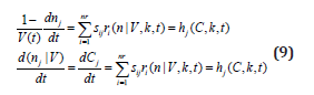
where notations are the followings: C(j) = (cell-)species “j” concentration; V = system (cell cytosol) volume; n(j) = species “j” number of moles; r(j) = jth reaction rate; s(i, j) = stoichiometric coefficient of the species “j” (individual or lumped) in the “I”- th reaction; t = time; k = rate constant vector; i =1,…,nr (no. of reactions)

h) It is self-understood that, as Max (Re (λ (i))) <0 is smaller as this cell QSS is more stable.

i) The key-species concentrations must be constant at QSS (homeostasis).

In fact, the cell metabolism optimality derives from the requirement to get a maximum growth / quick replication over a defined / limited cell cycle, by using minimum resources from the environment. These requirements are better illustrated by the 4 main characteristics of the cell systems, underlined in the (Outline 1).

Outline 1. The main characteristics of cell systems. i) The dynamic character of species interactions and processes [115].

ii) The feedback/feedforward character of processes ensuring their self-regulation [116].

iii) Optimal regulation of cell syntheses with fastest reaction rates, smallest amounts of intermediates, and best P.I.-s (see the below section) [115], with fulfilling (iv).

iv) Consuming minimum of resources (nutrients/substrates), and cell energy (ATP, NADH, etc.), but with also fulfilling (v), v) Ensuring maximum reaction rates [109].

Amazing, but the first pioneers in dynamic modelling of biological systems were not the (bio)chemical engineers which are better trained in ‘translating’ from the ‘language’ of molecular biology to that of mechanistic (bio)chemistry, by preserving the structural hierarchy and component functions (Figure 29) and using the NSCT concepts/rules. The first dynamic models of some cell processes have been reported by electronics [117,118]. Later, such ‘electronic circuits-like’ models have been extensively used to understand intermediate levels of regulation [1,2,4,5,119,120], but they failed to reproduce in detail molecular interactions with slow and continuous responses to perturbations and, eventually, they have been abandoned. However, the electronics underlined the main characteristics of the cell systems given in (Outline 1), which must be included in any cell dynamic simulation model. All these cell metabolic characteristics will be accounted for in all the subsequent cell in-silico WCVV simulators based on extended/ reduced mathematical models. All these characteristics are in fully agreement with the Darwin theory “Living organisms have evolved to maximize their chances for survival. It explains structures, behaviors of living organisms.” [108]. From such very incipient efforts to in-silico (math model-based) design of GMO-s, 40 years latter pointed-out the tremendous advanced in the systems Biology, and in the in-silico simulate the cell metabolism aiming to design GMO-s, or even tissues, by means of computational systems biology [118,121-122].

A review of mathematical model types (including the WCVV models) used to describe metabolic processes is presented by [1,2,4,5,28,73]. Each model type presents advantages but also limitations. Roughly, to model the complex metabolic regulatory mechanisms at a molecular level, two main approaches have been developed over decades: a structure-oriented (topological) analysis, and the dynamic (kinetic) models [1,2,4,5,78,123]. Each theory presents strengths and shortcomings in providing an integrated predictive description of the cellular regulatory network, as briefly reviewed by Maria [1,2,4,5,73], as follows. Structure-oriented analyses or topological models ignore some mechanistic details and the process kinetics and use the only network topology to quantitatively characterize to what extent the metabolic reactions determine the fluxes and metabolic concentrations [108]. The so-called ‘metabolic control analysis’ (MCA) is focus on using various types of sensitivity coefficients (the so-called ‘response coefficients’), which are quantitative measures of how much a perturbation (an influential variable) affects the cell-system states [e.g. reaction rates, metabolic fluxes (stationary reaction rates), species concentrations] in a vicinity of the steadystate (QSS). The systemic response of fluxes or concentrations to perturbation parameters (i.e. the ‘control coefficients’), or of reaction rates to perturbations (i.e. the ‘elasticity coefficients’) must fulfil the ‘summation theorems’, which reflect the network structural properties, and the ‘connectivity theorems’ related to the holistic (whole-cell, WC) properties of single enzymes in connection to the system behaviour.

MCA methods can efficiently characterize the metabolic network robustness and functionality, linked with the cell phenotype and gene regulation. MCA allows a rapid evaluation of the system response to perturbations (especially of the enzymatic activity), possibilities of control and self-regulation for the whole path or some subunits. Functional subunits are metabolic subsystems, called ‘modules’, such as amino acid or protein synthesis, protein degradation, mitochondria metabolic path, etc. [80]. Because living cells are self- evolutionary systems, new reactions recruited by cells together with enzyme adaptations can lead to an increase in the cell biological organization and to optimal performance indices. When constructing methods to optimize evolutionary metabolic systems, MCA concepts and appropriate performance criteria have been used, leading to: maximize reaction rates and steady-state fluxes; minimize metabolic intermediate concentrations; minimize transient times; optimize the reaction stoichiometry (network topology); maximize thermodynamic efficiency. All these objectives are subjected to various mass balance, thermodynamic, and biological constraints [108]. However, by not accounting for the system dynamics, and grounding the analysis on the linear system theory, topological methods present inherent limitations (see for instance some violations of stoichiometric constraints discussed by [124], or the use of modified control coefficients [125]. From the mathematical point of view, various structured (mechanism-based) dynamic models have been proposed to simulate the metabolic processes and their regulation, accounting for continuous, discrete, and/or stochastic variables, in a modular construction, ‘circuit-like’ network, or compartmented simulation platforms [1,2,4,5,79,123]. Briefly, the math models used by Systems Biology are of the following types, briefly described below [1,2,4,5,73].

I Deterministic continuous variable

Dynamic models can perfectly represent the cell response to continuous perturbations, and their structure and size can be easily adapted based on the available bio-omics information [1,2,4,5,28,73,108,123,126]. The deterministic continuous variable kinetic models present many advantages, as previously mentioned. Besides, it is to underlined the huge advantages coming from the used concepts, rules, and algorithms of BCE, and of the NSCT, as discussed in the Part-1 of this work, and by [1,2,4-7,73,87,88], and briefly represented in (Figure 4 & Figure 5) of Part-1 of this work). The classical approach to developing deterministic dynamic models is inspired by the CBE rules, and is based on a hypothetical reaction mechanism, kinetic equations, and known stoichiometry. This route meets difficulties when the analysis is expanded to large-scale metabolic networks of the CCM (Figure 1 & Figure 2) because the necessary mechanistic details and the standard/structured kinetic data at a cell species level necessary to estimate the MSDKM model rate constants are difficult to be obtained. However, advances in genomics, transcriptomics, proteomics, and metabolomics, lead to a continuous expansion of bioinformatic databases, while advanced numerical techniques, non-conventional estimation procedures, and massive software platforms reported progresses in formulating such reliable cell models. Valuable structured dynamic models, based on cell biochemical mechanisms, have been developed for simulating various (sub)systems [1,2,4,5,73].

II Boolean (discrete) variable models

Such models work with topological structures of the GRC-s. An example is displayed in (Figure 5) [77,123]. Due to the very large number of states O (103–104), and O (103) of transcriptional factors (TF) involved in the gene expression, such GRC models are organized in clusters, modules, of a multi-layer organization (Figure 5) [123,127]. In the Boolean/binary modelling approach, variables can take only discrete values (usually 0, and 1). Even if less realistic, such an approach is computationally tractable, involving networks of genes that are either ’on’ (1), or ’off’ (0) (e.g. a gene is either fully expressed or not expressed at all; Figure 5) according to simple Boolean relationships, in a finite space. Such a coarse representation is used to obtain a first model for a complex bio-system including many components, until more detailed data on process dynamics becomes available. “Electronic circuits” structures (see an example in (Figure 10-right), from [119,120]) have been extensively used to understand intermediate levels of regulation, but they cannot reproduce in detail molecular interactions with slow and continuous responses to perturbations, and they offer any information on the process / species concentration dynamics.

II Stochastic variable models [128-130]

Stochastic models replace the ‘average’ solution of continuousvariable (deterministic) ODE kinetics (e.g. species concentrations time-trajectories) by a detailed random-based simulator accounting for the exact number of molecules present in the system. Because the small number of molecules for a certain species (present in traces in a cell) is more sensitive to stochasticity of a metabolic process than the species present in larger amounts, simulation via continuous models sometimes can lack of enough accuracy for random process representation (as cell signalling, gene mutation, etc.). In such cases, Monte Carlo (stochastic) simulators are used to predict individual species molecular interactions, while rate equations are replaced by individual reaction probabilities, and the model output is stochastic in nature. Even if the required computational effort is extremely high, stochastic representation can be useful sometime to simulate the cell system dynamics by accounting for many species of which spatial location is important, or for a large distribution of concentrations [128-130] (Figure 10- left).

IV Mixed state-variable models [59,60,123].

Such cell (kinetic) models try to take advantage of each of the model type (I-III) mentioned above. The multiple advantages of the WCVV modelling framework are discussed, and exemplified by Maria [1,2,4-9,73,86,87]. In short, the novel modelling concept/framework WCVV proposed, extrapolated, and widely promoted in a large number of applications by Maria [1,2,4-9, 12-15,73,76,84,87,88] to derive cell kinetic models, in a holistic approach, ensures cell processes homeostasis, and the individual/ holistic GRC regulatory properties, by including in a natural way constraints related to the cell system isotonicity, and the variablevolume in relationship to the species reaction rates, and the lumped proteome/ genome replication [1,2,4-9,12-15,73]. Such an isotonicity constraint is required to ensure the cell membrane integrity, but also to preserve the homeostatic properties of the cell system, not by imposing ’the total enzyme activity’, or the ’total enzyme concentration’ constraints used by the classical (default) constant-volume cell modelling approach (WCCV). As proved by [6], compared to the classical WCCV models, the WCVV novel modelling framework is leading to more accurate simulations of cell metabolic effects, such as: relationships between the external conditions, species net synthesis reactions, osmotic pressure; the cell content (ballast) influence on smoothing the continuous perturbations in external nutrient concentrations; a more realistic representation of GERM regulatory modules and GRC-s, etc. At the same time, it is to highlight that the WCVV holistic cell modelling framework, which was proposed, deeply analyzed, and widely promoted in a large number of applications in bioengineering and bioinformatics by Maria [1,2,4-9,12-15,73,75,76,84,88] is proved to be more accurate and present a large number of advantages, as shortly summarized in (Table 2).

V Lumping MSDKM models

When the WCVV holistic MSDKM cell models are too extended to allow a quick use for biological reactor simulations/ optimization, or for in-silico design of GMO, then reduced kinetic models of cell CCM-metabolic syntheses, and of GRC-s can be obtained from the extended ones by applying specific kinetic model reduction/lumping numerical/analytical algorithms reviewed by [2,4,76,88,131,132]. The reasons of sometime using lumped WCVV holistic MSDKM cell models are given in (Figure 14). However, it is to mention that, even if computationally very convenient, the reduced (with lumped reactions and/or species) WCVV holistic MSDKM cell models presents a significant number of advantages, but also a couple of inherent disadvantages, reviewed in (Figure 12), and [2,4,5,76,88,131,132]

2.3.4. Modelling individual GERM-s under WCVV formulation

In order not to overly complicate the MSDKM or HSMDM models that also include GRC-s, it is necessary to have a “library” of kinetic models to represent individual GERM-s, to be used for build-up GRC-s of desirable properties (e.g. genetic switches, operon expression, genetic amplifiers, etc.; see Part-1 of this work [4,5]. As an example, see the case study with the mercury-operon expression in Part-4 of this work. Obviously, the selection of the most suitable GERM to be included in the GRC chain depends on its regulation performances, that is, the so-called self-regulation performance indices (P.I., see the below section), related to the GERM type. This chapter briefly presents the main GERM-s models proposed by Maria [1,2,4,5,73,93] used in the construction of HSMDM-s, in terms of the reduced reaction scheme, kinetic model, and their associated P.I.-s.

a) The modular approach

As experimentally proved in the literature (reviews [1,2,4,5,73]), the GRC-s (or GRN-s) „that control the synthesis of all proteins (enzymes) in the cell, present a modular construction, every operon (a cluster of genes under the control of a single promoter) including a variable number of interacting GERM-s. However, it is well-known that one GERM interacts with no more than the other 23-25 GERM-s [91], while most GERM structures are repeatable. Consequently, when developing the GRC analysis and reaction schemes / kinetic model, the modular approach is preferred due to several advantages: (i) A separate analysis of the constitutive GERM-s in conditions that mimic the stationary or perturbed cell growth; (ii) The GERM modules are then in-silico linked to construct the target GRC of an optimized regulatory efficiency that ensures key-species homeostasis and cell network holistic properties (Figure 13,14 & Figure 5). (iii) In-silico investigations of GERM-s and GRC-s characteristics focus on the tight control of gene expression, the quick dynamic response, the high sensitivity to specific inducers, and the GRC robustness (i.e. a low sensitivity vs. undesired inducers). Such advanced regulatory structures must ensure the homeostasis (quasi-steady-state, QSS) of the regulated key-species concentrations, and quick recovery (with a trajectory of minimum amplitude) after a dynamic (impulselike) or stationary (step-like) perturbation (Figure 11) of one of the involved metabolites or nutrients [1,2,4,5,73,93] (Figure 15 & Figure 16). To model complex GERM-s, intensive efforts have been invested over the last decades, and various types of dynamic models have been proposed, both in a deterministic [28, 48,50,85,86,95- 97,113], or stochastic approach [76,85,91,105,113]. See also the reviews [49,75,106,133] concerning structured deterministic models with continuous variables, built-up from time-series experiments [107,134]. However, to not complicate the resulted simulation model when coupling GERM chains in complex GRC-s, simple (lumped) GERM dynamic models have been proposed and investigated by various researchers [1-5,12-14,28,75,81,86,96- 98,106], as displayed in (Figure 4), with Hill-type [75,86,98,118], or pseudo-Hill-type activation [1,2,73,86]. See also the reviews [1,2,4,5,12-15,73,86,98].

b) The GERM library

To make this rule easier, Maria [1,2,4,5,73,93] has elaborated a library with reduced representations of GERM types (Figure 3) to be used for every case. Of course, these individual GERM modules differ as regulatory efficiency, as quantitatively expressed by their regulatory performance indices (P.I.) defined in the below section, in response to stationary or dynamic perturbations (Figure 11) into the cell, transmitted from the environment. These simplified deterministic models of lumped GERM and structures have been proved to adequately represent complex GRC–s (such as genetic-switches in Figure 5, or the mercury operon expression in Figure 6). The simplest GERM structure with one regulatory element is those denoted by [G(P)1], or one of a better regulatory efficiency [G(PP)1], with dimeric TF = PP (Figure 4). The generic [G(P)1] regulatory module (schematically represented in (Figure 17-down-right & Figure 3-the row-up & Figure 8) refers to the synthesis of a generic protein P and the simultaneous replication of its encoding gene G. The lumped [G(P)1] model includes only one regulatory element (a so-called “effector”, that is a fast ’buffer’ reversible reaction G + P <===> GP (inactive) (Figure 3), aiming at controlling the P synthesis rate and its homeostatic QSS level. The following notations have been used: G = active part of the gene encoding protein P; GP = inactive part of the gene encoding protein P; MetG, MetP = lumped DNA and protein precursor metabolites, respectively. The lumped ODE kinetic model of [G(P)1] are presented in (Figure 8) in both novel (correct) WCVV, and in the default (incorrect) WCCV modelling alternatives.

In such a generic lumped construction, the protein P and its encoding gene G mutually catalyses the synthesis of each other (that is cross-catalysis). The protein P is the ’control node’ playing multiple roles in such a simplified lumped representation. Thus, P is a permease facilitating the import of nutrients NutG, NutP in the cell, but also a metabolase converting the nutrients into precursors MetG and MetP of the G and P synthesis respectively. Protein P is also a polymerase catalyzing the gene G replication. And, finally, the protein P is also a transcriptional factor (TF) by dynamically adjusting the catalytic activity of G by means of a very rapid ’buffer’ regulatory reaction [G + P <===> GP (inactive)]. When P is produced in excess, it reversibly inactivates more amount of G, which, in turn, will slow-down the P synthesis. When P is produced in too low amounts, the regulatory process goes backwards.

The module nomenclature used in (Figure 3) for the GERM lumped regulatory modules, is those proposed by [73,93,94] is those of 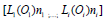. It includes the assembled regulatory unit . One unit ’i’ is formed by the component L(i) (e.g. enzymes or even genes G, P, M, etc.) at which regulatory element acts, and ni =0,1, 2… number of ‘effectors’/TF, generically denoted by species O(i) (that is ‘effectors’ like P, PP, PPPP, R, RR, RRRR, etc) binding the ‘catalyst’ L. For instance, a [G(P)2] unit of (Figure 3) includes two successive binding steps of G with the product P, that is: G + P <===> GP + P <===> GPP, all intermediate species GP, GPP, being inactive catalytically, while the mass conservation law is all time fulfilled, i.e. Such a representation accounts for the protein concentration diminishment due to the cell-growth dilution effect but could also include protein degradation by proteolysis. It is also to observe that such GERM lumped models try to account essential properties of the gene expression, that is a highly self- / cross- regulated and mutually catalyzed process by means of the produced enzymes / effectors. As depicted in (Figure 3 and Figure 8) for the [G(P)1] simplest regulatory module case, the protein P synthesis is formally catalysed by its encoding gene G. In turn, P protein lump catalyses the G synthesis, but also modulates the G catalyst activity via the fast-buffering reaction: G + P <===> GP. Even if such generic [G(P)1], [G(P)2], or [G(PP)1] regulatory modules are in reality more complex, by including a larger number of reactions and/or species involved in the regulation of the a target gene expression [1,2,4,5,86,98], it was proved (see the case study with the mercury operon expression in the Part-4 of this work) that such a reduced GERM model can satisfactorily reproduce the dynamics of complex GRC-s in MSDKM or HSMDM models.

As proved by Maria [1,2,4,5,76,86] these simplified formulations of various GERM types in (Figure 3) implicitly ensure an effective homeostatic regulation of the gene expression and G/P mutual autocatalysis of their synthesis. Cells are regulated such that their components are maintained at relatively invariant concentrations despite the presence of inherent external/internal perturbations. Recently, the effectiveness of various simplistic regulatory mechanisms in maintaining protein homeostasis in the presence of perturbations have been evaluated by [1,2,4,5,84,86,94,135]. Some of these representative GERM mechanisms, representatives of which are shown in (Figure 18), reflect the regulation of the synthesis (transcription and translation) and decay of a generic protein P. Both processes are required to maintain the protein [P] concentration at a nominal steady-state [P]ns (ns = nominal steadystate, QSS). It is self-understood that synthesis of a protein involves many species (components), but in such lumped representation of GERM mechanisms, all except for the generic key-gene G encoding P (and in some cases the corresponding mRNA) are ignored and assumed to be present at constant concentrations and included in the model species lumps. In the ’control’ mechanism, denoted by [G(P)0], P is synthesized in a single reaction catalyzed by G (Figure 18, mechanism no. 1). In a default constant-volume WCCV (incorrect) model [94,136] considered a P degradation reaction of a first order in P. In real cells, proteins are generally stable, and so these fictitious decay terms reflect the cell dilution (’D’) caused by volume expansion as cells grow, as correctly modelled by the WCVV approach, that is eq. (3a-b), eq.(4a-b), eq. (5).

Other GERM models include negative feedback regulatory elements in various combinations. For instance, in the [G(P)1] model, one P binds G reversibly (Figure 18, mechanism no. 2). The resulting GP form is catalytically inactive, and so this relationship serves to regulate the protein synthesis. The dissociation equilibrium constant is set to equal [P]ns, ensuring that [G]ns = [GP]ns at [P]ns. Thus, when [P] > [P]ns, then P tends to bind more G and to «attenuate» the protein synthesis. Conversely, when [P] < [P]ns, then P tends to dissociate from GP, thereby increasing the rate of protein synthesis. This reaction mechanism, even lumped, leads to a satisfactory regulatory effectiveness of the GERM. Other more effective GERM mechanisms, like [G(P)1; M(P)1] distinguish between transcription and translation (Figure 18, mechanism no. 3), being closer to reality. In it, G catalyzes the synthesis of M (i.e. mRNA), and M catalyzes the synthesis of P. Also included is the reversible binding of P to M, stimulating the degradation of M to form M’. In the mechanism [G(PP)2], two copies of a PP dimer (playing the role of a TF) reversibly bind G (Figure 18, mechanism no. 4), mimicking the multiple binding of transcription factors which often bind promoters as oligomers and in multiple copies. As revealed by (Figure 19), the efficiency of all these four (no. 1-4) GERM-s mechanisms is very good when coping with a dynamic perturbation, that is a 10% negative perturbation (impulse-like) of [P] from [P]ns = 1000 nM, to [P]ns = 900 nM. It is to remark that the species recovering trajectories are as faster as the GERM efficiency schema is « better » (in terms of P.I.-s), that is in the relative order:

[G(PP)2] > [G(P)1; M(P)1] > [G(P)1] > [G(P)0]

It was proven [1-5] that the P.I .-s of GERM-s increase nearly linearly with the number n(i) of effectors (P, PP, PPPP, etc.) acting in the i-th allosteric unit [L(i)(O(i))n(i)], or the number of buffering reactions applied at various levels of the gene expression control. Such an observation is valid for both dynamic and stationary P.I.-s of the (Table 3). Roughly, the P.I .-s improves ca. 1.3-2 times (or even more) for every added regulatory unit to the same GERM type of Figure 3.

A more detailed discussion on this subject is offered by Maria [1,2,4,5, 8,9,93], by highlighting the role of the number of effectors on the GERM P.I.-s (Figure 15, and the below section).”

c) Rate constant estimation in WCVV models of GERM-s and GRC-s

In the WCVV ODE differential models of GERM-s or GRC-s, due to the lack of standard/structured kinetic data, the large numbers of rate constants are estimated by a more elaborated numerical rule. If the estimation problem can be splitted between those referring the MSDKM ODE model concerning the CCM, and those referring the attached GRC, then, one can proceed first to the estimation of GRC- ODE kinetic models, and then those related to the CCM (see an example in the case of the bioreactor simulation/ optimization for the tryptophan (TRP) production, in the Part-3 of this work). For a given GERM or a GRC, ODE kinetic model, if the stationary cell species concentration vector Cs is known from the experimental data (for the all individual or lumped components considered in the kinetic model), then the rate constant vector k (and even unknown Cs) of the kinetic model eq. (3A-B) results by solving the nonlinear algebraic set eq. (8), by using the effective MMA procedure of Maria [131,136-138], with imposing several physical significance constraints. The solving rule also includes the built-in procedures of the MapleTm symbolic computing platform. As the (RT/π) term is known from the initial condition eq. (6), and the number of model parameters is usually higher than the number of observed cell species, supplementary optimization rules can be applied to determine some rate constants, by imposing optimum regulatory criteria of GERM-s (see below P.I.-s section, [1,2,4,5,8,9]), such as the minimum recovering time of the stationary concentrations (homeostasis) after a dynamic (‘impulse’-like) perturbation in a key-species (Figure 11) & Figure 16), and eqn. (10) [73]. Of course, the use of an effective NLP (nonlinear programming) solver plays an essential role in this model parameter estimation process [131,136-138].

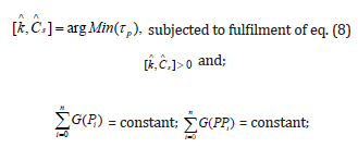
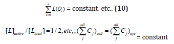
With the following notations: superscript ’^’ = estimated value; p τ = the recovering time of [P]s with a tolerance of 1%[P] s after applying a 10%[P]s impulse perturbation of its stationary value [P]s ; component Li (e.g. enzymes or even genes G, P, M, etc.) in a GERM is those species at which the regulatory element O, TF, R acts (see [1,4,73,75,76,]). To estimate, other regulatory global properties can also be used together with the NLP estimation problem constraints eqns. (6,8,10) [73,74,131,138]. The reverse reaction rate constants in the rapid buffer reactions of GERM-s, of type G+P <-------> GP, are adopted at values five to seven orders of magnitude higher than D in eq. (3A-B) (see the proof of Maria [86]). That is because fast buffering reactions are close to equilibrium and have little effect on metabolic control coefficients. Consequently, rate constants of such rapid reactions are much higher than those of the core synthesis and dilution rates.” Besides, additional constraints should be imposed to the GERM-s kinetic modules to ensure a quick dynamic regulatory efficiency (effective P.I.-s) based on effective transcriptional factors (TF-s, of P, or P -polymer types, e.g. PP. PPPP, etc.) [1,2,4,8,9,14,73]. Because the problem of estimating reaction rate constants for such MSDKM hybrid structured kinetic models with continuous variables [of mixed ODE-algebraic type, eq.(3A-B); eq.(4A-B), eq.(5) ] in the presence of constraints is one of NLP (nonlinear programming) type [131], with a convex search field and a function multi-modal objective, its solution is difficult to be obtained, even if highperformance numerical optimization algorithms (included in commercial mathematical software, e.g. MatlabTM) are used in this respect. Therefore, the feasible global solution for such estimation problems was found by applying only very efficient numerical solvers, such as MMA optimization procedure of Maria [136,137].

Once the GERM/GRC kinetic model rate constants (and, if necessary, the stationary values of some metabolic intermediates concentration) have been estimated, estimation of the whole CCM modular kinetic model MSDKM can be easier performed by adjusting (if necessary) some rate constants of the GRC included in the CCM model. See the example of E. coli CCM MSDKM model estimation together with the adjustment of the TRP (tryptophan)- operon kinetic model in Part-3 of this work. A similar example presented in Part-4 of this work concerns the HSMDM model for the mercury uptake in cloned E. coli cells.

2.3.5 GERM-s regulatory performance indices (P.I.) under WCVV formulation

”As proved in previous works [1,2,4,5,8,9,73,75,76,93], the performances indices (P.I.-s) of GERM–s of [G(P)n] type in (Figure 3), are as better as the number ’n’ of buffer reactions increases (Figure 15 & Figures 18,19), the right GERM choice when constructing a GRC being case dependent (see [12-14] as an example). Also, Maria [1,2,4,5,] proved that, when the a generic protein P is also acting as a TF (directly, or indirectly, by influencing the TF synthesis), its efficiency is better if it is present in a dimeric form (PP), in GERM-s of [G(PP)n] type in (Figure 3-middle row, Figure 15 , Figure 20), acting at both G and M levels of the expression (middle and down-rows of Figure 3), thus developing a cascade control scheme of the expression where transcription and translation regulatory steps are separately considered, that is GERM-s of [G(PP)n; M(PP)n’] type. Perturbations of the species steady-state (QSS, homeostatic) concentrations are caused by changes in the cell environment. In a GERM case, these processes tend to increase or decrease the key-protein stationary level [P] s. These processes occur in addition to those of the ‘‘core’ system focus on the genome (and all G/P pairs) replication over the cell cycle. GERM or GRC regulatory performance indices P.I.-s are of two types [1,2,4,5, 8,9,74,76,77,94]: stationary or dynamic, according to the perturbation type (Figure 11 and Figure 16). Briefly the P.I.-s are presented in the (Table 3), together with the associated optimization objective (goal), for a general nonlinear dynamic cell model described by eq. (3A-B).

See also an intuitive display in (Figure 11 & Figure 21) Detailed information is given by Maria [1,2,4,5,73,93]. The monodromy matrix A, necessary to express the species QSS-level stability ’strength’ is evaluated together with the cell process ODE model eqn. (3A-B), by using the following ODE differential set:

Detailed explanations of P.I.-s presented in (Table 3) are given by [1,2,4,5, 8,9,73,76,93]. In short, P.I.-s are the followings:

A) Stationary P.I.-s are defined as response to a stationary perturbation (Figure 11), that is transition from a QSS concentration to another QSS following a ’step’-like perturbation of one cell component concentration. These stationary P.I.-s are expressed in the following ways:

i. Transition time necessary for each GERM component to return to their stationary concentration (QSS) after a steplike perturbation in one component of the regulatory module (individual or lumped component.

ii. Responsiveness to exo/endogeneous signaling species of the analysed GERM or GRC can be represented by the small transient times necessary for a species ’j’ QSS-level to reach a new QSS (with a certain tolerance, usually 1-5%) after applying a stationary external stimulus [98]. Consequently, the P.I. measure of the GERM efficiency to move fast to a new QSS is given by the duration of the transition time τP (in the case of P-species in Figure 11) necessary to a certain component to reach the new steady-state concentration.

iii. Stationary efficiency This stationary P.I. is related to the small sensitivities S(C(i); NutP(j)) of the key-species levels C(i) vs. changes in the external nutrient levels NutP(j) and is simply denoted by . These sensitivities are computed from solving a sensitivity nonlinear algebraic set obtained by assuming QSS conditions eqn. (8) of the ODE kinetic model eqn. (3A-B), and known nominal species stationary concentrations Cs. Then, differentiation of the steady-state conditions eqn. (8) leads to the evaluation of the state sensitivity vs. nutrient levels, that is S(C(i); Nut(j)) = ∂Ci / ∂Nut(j). See the details of Maria [1,2,4,5, 73,93].

iv. The steady-state Cs stability strength This GERM property is related to the strong capacity of the regulatory systems to ‘resist’ to large external / internal perturbations, thus maintaining the system steady-state Cs, and then determining very quick recovering paths. As with all other P.I.-s, this regulatory property is related to the GERM system characteristics (structure, properties). Basically, as Max (Re (λ (i))) <0 is smaller as a Cs (QSS) is more stable. Here, the eigenvalues λ (i) of the Jacobian matrix 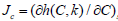, (see its definition before eqn. (9)) are evaluated at a checked QSS of the species concentration vector (Cs). In a more systematic approach, the steady-state Cs stability strength. can also be associated to an index against periodic oscillations of the key-species synthesis. This index can be evaluated from the linearized form of the system ODE model, by calculating the monodromy matrix A(T) after a checked period ’T’ of time [93], by using eq. (11). For a stable Cs, i.e., < 1 as are smaller, as the stability of the Cs state is stronger, and that QSS recovers faster after a small dynamic perturbation. Here, denotes the eigenvalues of the A(T) matrix, while I = the identity matrix. In other words, QSS stability strength involves: Min (Max (Re (λ (i))), with Re (λ (i)) < 0 for all ’i’, and Min < 1.

B) Dynamic P.I: is defined in relation to the GERM/ GRC response to a dynamic perturbation (Figure 11), that is the recovery of the QSS following an ’impulse’-like perturbation in the stationary concentration of one of the cell components. Dynamic perturbations refer to instantaneous changes in the concentration of one or more cell components that arise from a process lasting an infinitesimal time (impulse-like perturbation). After perturbation, the system recovers and returns to its stable nominal state QSS (see Figure 11 & Figure 16 for a generic P-protein synthesis in the case of the simplest [G(P)1] regulatory module. The computed recovering time τ(rec, j) necessary to each component ’j’ to reachback their stationary concentration (with a tolerance of 1-5% proposed by Maria [73]) may differ from one species to another depending on how effective their GRC are where it is involved.

In fact, the recovery rates of the species QSS (homeostasis) are holistic properties of the cell GRC-s, by involving all interactions within the cell-system, rather than of the individual elements thereof [108]. In terms of the evolution and stability of species QSS concentrations included in a dynamic cell system expressed by an ODE model eq. (1A-B), or eq. (3A-B), and eq. (4A-B), eq. (5), these properties can be evaluated from the analysis of the eigenvalues λ(i) ( i = no. of species) of the linearized ODE kinetic model Jacobian matrix , of elements J (i, k) = ∂ h(i)(C,k) / ∂ C(k) defined before eqn. (9). If small perturbations of a steady state Cs are considered then, this steady state is asymptotically stable if the real parts of the Jacobian eigenvalues are all negative, that is Re (λ (i)) <0, for all ’i’ [108,139,140]. If the system is stable then, it reaches the same QSS after cessation of a dynamic impulselike perturbation, or it reaches another QSS after cessation of a stationary step-like (stationary) perturbation (Figure 11). Here it is to mention the works of Maria [1,2,4,5,73,93], and of Sewell et al. [135], proving that the optimum concentrations in the ‘buffering’ reactions of GERM-s involving the active and inactive forms of the ’catalyst’ ensuring the maximum regulation dynamic efficiency vs. perturbations are those of [G] = [GP], [Gi]=[GiPjPj], of [M] = [MP], [Mi]=[MiPjPj], etc. (for the GERM-s types displayed in Figure 3). The main dynamic P.I.-s discussed by [1,2,4,5,8,9,73,93] are the followings (Figure 11):

a) Recovering time (t(rec,j), or simply t(j)) necessary to each GERM’s component to return to their stationary concentration (QSS) after an impulse-like perturbation in one component (see Figure 11, and Figure 16 for a generic P-protein synthesis in the case of the simplest [G(P)1] regulatory module). In other words, this P.I. refers to the GERM efficiency to fast recover the key-species stationary Cs, that is a short time t(j) necessary to the species ’j’ to recover its steady-state concentration (with an assumed tolerance of 1%, as proposed by [73]). As an example, in (Figure 16 & Figure 22) is proved how a simple generic GERM of [G(P)1] type presents a better dynamic efficiency compared to the simplest [G(P)]0 gene-expression module. Thus, the stationary [P] s and [G]s is recovered faster after an impulse perturbation in the [P]s, that is a -10% decline of [P]s at an arbitrary time t=0 [8,9]. As another example, in (Figure 23) is presented how the dynamic regulatory efficiency (that is the recovering time of the key lumped species G/P to reach their QSS) depends on the GERM’s structure, and its number of effectors (TF-s). Thus, the regulatory efficiency increases in the order:

[G(P)]0 (’1’) < [G(P)1] (‘2’) < [G(P)1; M(P)1] (’3’) < [G(PP)2] (’4’)

b) Recovering rate RD (Table 3) is those necessary to each GERM component to return to its stationary concentration (QSS) after cessation of an impulse-like perturbation in one component. As an example, in (Figure 15) is presented how RD depends on the GERM structure, and its number of effectors (TF) (see their nomenclature in Figure 3). The recovering rate RD reflects the recovering properties of the regulated key-P synthesis by the GERM modular system. In a simpler way, the species ’j’ recovering times τ (j) ~ 1/RD and trajectories Cj(t) can be obtained by simulation, that is by simulating the GERM system dynamics [with using the GERM ODE model eqn. (3A-B, 4A-B, 5), or eqn. (8) ] after applying a small impulse perturbation of the species steady-state of +/-10% Cj,s and determining the recovering time until the steady-state Cj,s is reached with a 1% tolerance [1,2,4,5, 8,9,73]. Species recovering trajectory and amplitude are both very important (Figure 15 & Figure 23). As proved by Maria [1,93], GERM-s display very different recovering trajectories and amplitudes according to their reaction parhway structure (Figure 15). The most effective are the GERM types ensuring the smallest amplitude of the recovering pathway, thus not disturbing the other cell metabolic processes. As underlined by Maria [1,93], the recovering trajectories in the G/P phase plane are more ’linear’-like for the efficient GERM-s, by presenting a lower amplitude, thus not disturbing other cell reactions and regulatory circuits.

c) Regulatory robustness. The regulatory robustness of a GERM dynamic model is defined by Maria [1,4,8,9,73] as being the property to realize (Min) ∂R_D/∂k , where RD denotes the keyspecies recovering rates of their QSS, after cessation of a dynamic perturbation, while ’k’ is the vector of the rate constants of the GERM model (depending on the micro-organism type). This P.I. can be considered a systemic regulatory property if GERM species levels are able to modify the apparent reaction rates. In fact, the cell metabolic network robustness and functionality are linked to the cell phenotype and gene regulation scheme (depending on each individual expression).

d) Species interconnectivity in a GERM modular regulatory schema of reactions can be viewed as a degree to which they ‘assist’ each other, and ‘cooperate’ during the GERM system regulation to realize their optimal regulatory P.I.-s. Cell species connections appear due to common reactions, or common intermediates participating to the chain of reactions, or from the common cell volume to which all cell species contribute (under constant osmotic pressure, eq. (3A-B, 4A-B, 5, 6), and WCVV model hypotheses of (Table 2). Vance et al. [141] reviewed and proposed several quick experimental/computational rules to check a reaction schema via species inter-connectivity’s. By inducing experimental perturbations to a (bio)chemical system, by means of concentration tracers, or by fluctuating the inputs of the system, one can measure the perturbation propagation through the consecutive/parallel reaction pathway. Then, various techniques can determine the ’distance’ among observed species and then, specific rules can be used to include this information in elaborating a reaction schema [8,9,12-14,73,75,86,98]. In this respect, Maria [73,75,76,86,98] proposed an approximate measure of species interconnectivity related to the species recovering-times after a dynamic perturbation, that is: AVG (t(j)) and STD (t(j)), i.e. the average and the standard deviation of the species individual recovering times t(j), respectively. As AVG and STD are larger, the cell GERM/GRC dynamic regulatory effectiveness is lower, species less interconnected, and components recover more disparately (scattered recover times). The higher the number of effectors and buffering reactions, the better these dynamic regulatory indices of the GERM are [1,2,4-9,12-15,48,73,75,76,86,93,98].

e) Cell sub-system QSS stability (and of a GERM) refers to the cell system’s capacity to recover a QSS (that is the homeostasis of a balanced cell growth) after cessation of any dynamic perturbation. Such a property can be better pointed-out by analysing the QSS and eqn. (8) derived from the dynamic GERM ODE model eqn. (3A-B). The stability property can be evaluated from the analysis of the eigenvalues λ (i) (i = no. of species) of the linearized model Jacobian matrix of elements J(i,k) = ∂h(i) (C,k) /∂C(k) defined before eqn. (9). The QSS is asymptotically stable if the real parts of the Jacobian eigenvalues λ (i) are all negative, that is Re (λ (i)) <0 for all ’i’ [108,139,140,142]. If the system is stable then, it reaches the same QSS after cessation of a dynamic impulse-like perturbation, or it reaches another QSS after cessation of a stationary step-like perturbation. Here it is to mention two important observations:

i) A characteristic of the WCVV models including the Pfeiffers’constraint eq. (2), translated in eqn. (3A-B, 4A-B, 5, 6), is that they are always stable (intrinsic stability), because, as proved by Morgan et al. [92], always Max (Re(λ (i))) = -D [ see eq. (3A-B, 5)].

ii) By contrast, one fundamental deficiency of the classical/ default WCCV model (incorrect) formulation is the lack of the intrinsic stability of the cell system ODE dynamic model, because the WCCV models do not include neither the Pfeiffers’constraint eq. (2), nor an equivalent constraint to ensure the cell isotonicity and, consequently, its membrane integrity. It follows that, working under a classical WCCV modelling framework, the GERM regulatory mechanism for recovering the system homeostasis (illustrated in Figure 3, Figure 16 & Figure 23), is no longer working, and the dynamic ODE model becomes invalid, ineffective, and not applicable.

2.3.6. Some rules to link GERM-s when modelling GRC-s

When modelling a GRC consisting of a network of GERM-s, „there are two problems to be considered: (i). what types of GERM-s must be chosen from the library of (Figure 4-7) to match the individual gene expression characteristics, and (ii). what rules are to be applied for linking GERM-s to obtain the holistic regulatory properties of the GRC in the context of the cell balanced growth. A successful example of a HSMDM model is given in Part- 4 of this work, that is the case study referring to modelling the mercury-operon expression induced by the presence of mercury ions in the E. coli cell environment. The complex GRC was obtained by linking 7 individual GERM-s [1,2,4,5,12-15]. For this case study, the GRC-operon model including GERM-s of [G(PP)1] type, and their arrangement in a cascade control with feedforwards, and feed-back loops have been found to be the best ODE structured dynamic model able to adequately reproduce the experimental data. In fact, when developing a math (kinetic) cell structured ODE model linking a couple of GERM-s to construct a certain GRC to reproduce/simulate certain regulatory functions concerning the cell metabolism, there are several trends used in the in-silico analysis:

a) On one hand is the natural approach of using simple (lumped) GERM structures (see the GERM library of Figure 3) to reduce the large computational effort required to estimate the rate constants of the corresponding HSMDM model (that incorporate the GRC model), and for its quick simulation.

b) On the other hand, it is important to use effective and flexible GERM-s able to reproduce the individual enzymesynthesis, but also the holistic properties (P.I.-s) of the GRC mentioned in Table 3). Some examples are provided by Maria [4,5]).

c) To ensure the optimal efficiency of a resulted GRC, and their functions into the cell, Maria [1,2,4,5,73] elaborated a couple of rules to be followed, and accounted for, when linking GERM-s to form a GRC. This sub-chapter aims to briefly review the main linking rules.

i) Rule 1: The effect of the no. of regulatory effectors (n)

By definition, GERM models (see Figure 3, and the nomenclature given in section “The GERM library”) include an adjustable number of ’regulatory effectors’, that is: ’n’ for the [G(P)n] type, or [G(PP) n] series; ’n’ and ’n1’ for the [G(P)n; M(P)n1] series. As proved by Maria [73,76,93], and others [94], a quasi-linear relationship of the GERM module P.I.-s function of no. of regulatory effectors ’n’ can be derived for every GERM type, of the form (Notations: a(o), a(i) denotes the correlation constants related to a certain P.I., and module type). Here, P.I. denotes the regulatory performance index (chap. 2.3.5), such as RD, AVG (τ(j)), STD (τ (j)), stability strength, etc. Also, n(i) = number of effectors (P, PP, O, etc.) acting in the ’i-th’ allosteric regulatory unit [Li (Oi)n(i)]. This rule is maybe the most important, the above linear dependence being observed in the examples displayed in (Figure 20 & Figure 15). In short, Maria [4,5,73,75,76,86] proved the following GERM-s properties (see also Figure 20, Figure 15):

a) P.I. improves ca. 1.3-2 times (or even more) for every added regulatory unit to a GERM model of (Figure 3). Multiple regulatory units lead to an average recovering time AVG (τ(j)) of all GERM species much lower than the cell cycle duration ’tc’, under a constant logarithmic volume growing rate, D = ln (2)/tc. (see eqn. 4B)

b) Combinations of GERM regulatory schemes (with different effectors) can improve the regulatory P.I.-s.

c) Certain GERM regulatory modules reported an increased flexibility, due to ‘adjustable’ intermediate species levels. This is the case, for instance, of adjusting [M]s in the GERM modules of type [G(P)n; M(P)n1], or of adjusting [PP]s in modules [G(PP)n] of (Figure 3, Figure 15, Figure 20 & Figures 18-19). Optimal levels of these species can be set according to various optimization criteria, rendering complex regulatory modules to be more flexible in reproducing certain desired cell-synthesis regulatory properties (see the example given by Maria [98]).

ii) Rule 2: Ranging the number of transcription factors TF and buffering reactions

To select the suitable GERM structure that fits the available experimental (kinetic) data of the cell metabolism, the first problem to be solved is related to the number of buffering reactions of type:

necessary to be included in the model to obtain the desired optimal P.I.-s (Figure 3, Figure 23 & Figure 24) [86,98]. Evaluation of P.I.-s for a large number of GERM types (Figure 3) [1,2,4,5,12- 15,73,75,76,86,87,98,114] indicated that the dynamic regulatory efficiency of [G(P)n], or of [G(PP)n] modules is nearly linearly increasing with the number ’n’ of buffering reactions (following the above correlation given at the rule no. 1). Moreover, the plots of (Figure 15) reveal that P.I.-s increase is more pronounced in the case of GERM-s of [G(PP)n] model types, that use dimeric TF-s (that is PP instead of simple P). Also, GERM-s of type [G(P) n; M(P)n1] models that use a control scheme in cascade of the gene expression reported superior regulatory P.I.-s. Such a GERM module efficiency ranking according to the number of effectors concerns not only its dynamic regulatory efficiency, but also most of P.I.-s, as discussed in the previous section, such as (Table 3):

a) The stationary regulatory effectiveness.

b) The low QSS sensitivity vs. stationary perturbations.

c) Stability strength of the homeostatic QSS.

d) The shorter species recover trajectories in the G/P phase plane, and of a lower amplitude.

iii) Rule 3: The effect of the mutual catalysis in the G/P synthesis

One essential aspect of the [G(P)n], [G(PP)n], and [G(P)n; M(P) n1] kinetic models of GERM--s is the mutual catalysis of G and its encoding protein P synthesis. If one adds the WCVV modelling constraints eqn. (3A-B, 4A-B, 6, 8), and the requirement of getting a maximum dynamic responsiveness and efficiency by keeping [G]s = [G(P)]s = [G(PP)]s = …= [G(P)n]s, as discussed by Maria [1,2,4,5,73,75,76,93]. This direct and indirect link (via GP, GPP, etc., and the cell volume/osmotic pressure) of G and P syntheses ensures a quick recovering of both stationary [G]s and [P]s after any small perturbation of their QSS (stationary, homeostatic) concentration. To prove this in a simple way, one considers the synthesis of a generic G/P pair in a GERM of [G(P)1] type (denoted by ’2’), or a [G(P)0] type (denoted by ’1’) in (Figure 3 & Figure 23). After estimating the rate constants from solving the stationary model equations by using the homeostatic concentrations of (Figure 25, high ballast cell case), one determines the dynamic efficiency for each GERM by applying a negative 10% impulse perturbation in the [P]s = 1000 nM at an arbitrary time t=0. The obtained recovering trajectories of P and G obtained by model simulations are plotted in (Figure 16 & Figure 23). The plots reveal a satisfactory good regulatory efficiency of the [G(P)1] type of GERM, both G, and P species presenting relatively short recovering rates, and negligible for the other species. These plots reveal, in a simple way, the selfregulation of the G/P pair synthesis: after an impulse perturbation leading to the decline of [P]s from 1000 nM to 900 nM, the very fast buffering reaction G + P <===> GP leads to restore the active G, whose concentration quickly increases from 0.5 nM to [G] = 1.027 nM. Therefore, the synthesis rate of P increases leading to a fast P recovering rate which, in turn, contributes to the recovering of the G-lump steady-state. For comparison, as revealed by the results displayed in the (Figure 22), the dynamic efficiency of the module [G(P)0] is much lower, species recovering their QSS over longer transient times. Also, the species connectivity is better in the [G(P)1] case compared to [G(P)0], due to the reported smaller STD (τ (j)) (Table 3). Consequently, removal of the buffering reaction that automatically adjusts the ’catalytic activity’ of G, will:

a) Decrease the species inter-connectivity (by increasing the standard deviation of their recovering times).

b) Will increase the species recovering times.

c) Will increase the sensitivities of the species steady state vs. external nutrients (see sensitivity coefficients vs. NutG in Figure 22).

As expected, the P.I.-s of the GERM–s depend not only on (a) the no. of effectors (buffering reactions), but also on (b) the TF types (P, or PP), and even more (c) on the used control scheme (i.e. simple buffer reaction of G-activity, or in a cascade of buffer reactions, like the [G(P)n; M(P)n1] reaction schemes). To better exemplify these issues, one considers the same generic G/P gene expression example with the species homeostatic stationary concentrations given by of (Figure 25, high ballast cell case). For comparison, one considers GERM model types, of structures given in the (Figure 23), that is [G(P)0] without mutual catalysis, [G(P)1] with mutual catalysis and one buffering reaction, or [G(PP)2] with dimeric TF=PP, or even [G(P)1;M(P)1] with mutual catalysis and a cascade control via buffering reactions at both G and M levels. The rate constants have been estimated by solving the stationary form of the GERM model with the stationary concentrations (eq. (8)). Additionally, the requirement of getting a maximum dynamic responsiveness and efficiency, as discussed by Maria [1,2,4,5, 73,93], leads to adopt [M]s = [M(P)] s = 0.5 nM, and [G]s = [G(PP)] s = [G(PPPP)]s = 1/3 nM. The resulted recovering trajectories of the G and P species after a –10% impulse perturbation in the [P]s = 1000 nM at an arbitrary t=0, are comparatively presented in the (Figure 23). It is to remark that the incomplete [G(P)0] module reports the worst dynamic efficiency, with a very slow recovering rate after a dynamic perturbation in [P]s, as depicted in (Figure 23). Better performances are reported by the [G(P)1] module type. Even if a better regulatory efficiency is reported by the cascade control of separately considered transcription and translation of the [G(P)1;M(P)1] module, the best QSS recovering efficiency is reported by the [G(PP)2] module that uses two buffering reactions and a dimeric PP as TF, quickly synthesized in a small amount (of optimal level [PP]s = 0.01 nM determined together with the model rate constants to ensure an optimal P.I.). Due to such reasons, GERM-s modules of type [G(PP)2] will be preferred when buildup the GRC for the mercury-operon expression in one of the case studies of the Part-4 of this work.

All the above analyzed GERM-s have been modelled in a WCVV framework (eq. 3a-b, 4a-b, 5-8). For such WCVV kinetic models, it is to remark the way by which the variable cell-volume plays an important role to species inter-connectivity (direct or indirect via the cell volume to which all cell components contribute), within a certain GERM regulatory module or among linked modules. Even if species connectivity can be expressed in several ways [48,141], this index is directly dependent on how species in a GERM or in a GRC recover independently after perturbation. As the species connectivity increases, as they recover at a more comparable rate (or equivalently, over the same time), by ‘assisting’ each other to cope with a perturbation (see the comparison of species recovering times in Figure 22). By contrary, when the species are more disconnected, they recover in a more disparate way, and the GERM presents weaker P.I.-s. [reporting not only larger species recovering times τ (rec)(j), but also larger state sensitivities to external nutrients, see Table 3]. Thus, the mutual autocatalysis G/P appears to interconnect the GERM key-components such that they are regulated more as a unit than would otherwise be the case.

iv) Rule 4: The effect of cell system isotonicity

The positive effect of the isotonicity constraint eqn. (2, 3a-b, 4a-b, 5-8) of a WCVV cell model was proved by Maria [1,2,4,5,73].

By simulating the GERM species dynamics of a [G(P)1] model type, the effect of applying a –10% impulse perturbation in the key-protein homeostatic level [P]s = 1000 nM at an arbitrary time t=0, on the key-species (G, P) can be observed in (Figure 16), while species recovering times are given in (Figure 22). By contrast, in a classic (default) WCCV cell model formulation, when the isotonicity constraint is missing from the ODE dynamic model, the key-species do not recover after a dynamic perturbation (!). By contrast, as revealed by the performed simulations with the a [G(P)1] module, the system isotonicity imposes relatively short recovering rates for the key-species, and negligible for the other GERM species present in a large amount (that is the lumped nutrients and metabolites). By contrast, as proved by Maria [1,2,4,5,8,9,73], the WCVV models, with including the ’cell ballast’ effect, and the G/P mutual cross- and auto- catalysis, are more flexible and adaptable, thus better representing the cell adaptation to the environment changes.

v) Rule 5: The importance of the adjustable regulatory TF-s in a GERM

As proved by the example of (Figure 23), and those of [73,93], the use of dimeric TF-s, such as PP in [G(PP)n], instead of simple P in [G(P)n], is advantageous, as revealed by the following simulation results:

a) The dynamic regulatory efficiency increases in the order: [G(P)0] (no buffering reaction) < [G(P)1] (one buffering reaction) < [G(P)1; M(P)1] (cascade control and a buffering reaction at the M level) < [G(PP)2] (two buffering reactions, with dimeric TF= PP, in a small quantity). Some GERM modules reported an increased P.I. flexibility, due to ‘adjustable’ intermediate TF species levels. This is the case, for instance, of adjusting [M]s in the module [G(P) n; M(P)n1], or of [PP]s in the modules [G(PP)n]. Optimal levels of these intermediate species can be determined from matching various optimization criteria, rendering complex GRC-s to be more flexible in optimally reproducing certain desired cell-synthesis regulatory properties [1,4,5,8,9,98].

b) The dynamic regulatory efficiency (defined in Table 3, and in the section 2.3.5) decreases in the following order [1,2,4,5, 73,93]:

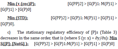
vi) Rule 6: The effect of the cell ballast on the GERM efficiency

When constructing simplified cell models of GERM-s/GRC-s by using the WCVV approach, it is important to know what the minimum level of simplification is to not essentially affect the holistic properties of the cell, and their key-functions (Outline 1). This paragraph proves why it is essential for a WCVV cell modelling approach to include all cell species, all forming the so-called ’cell ballast’, that is the sum of all species concentrations, even if they are explicitly or not accounted in the ODE mass balance of the GRC model. Basically, the isotonic constraint imposes that all species (individually, or lumped) to be accounted in the cell model, because species concentrations and rates are linked through the common cell volume eq. (2, 4A, 6). As proved by Maria [1,4,5,8,9,84], and (Figure 25), in such WCVV cell model constructions, the recovery rates are properties of all interactions within the cell system rather than of the individual elements thereof [108]. However, another important question related to the cell ballast and the isotonicity constraint refers to the degree of importance of the cell content (ballast) concerning the cell reactions, and their species QSS-levels ’resistance’ to dynamic/stationary perturbations (Figure 11).

In other words, the P.I.-s of a GERM, or of a GRC, are the same in a ’rich’ cell of high cell content (ballast), compared to those from a ’poor’ cell of low cell content (ballast)? The answer is no! To prove that in a simple way, one considers a GERM of a generic [G(P)1] type placed in an E. coli cell with two different nominal conditions given in (Table 4) for a high-ballast cell, and a lowballast cell. To not complicate these models, lumped gene and protein metabolites have been considered. Being present in a large amount (that is lumped [MetG] = 3E+6 nM and lumped [MetP]= 3e+8 nM), these components also play the role of cell ballast, their concentrations being set to values much larger than those of the other cell species. Simulations of Maria and Scoban [8,9], allowed obtaining the species trajectories, and their recovering times after a –10% impulse perturbation in the key-protein [P]s of 1000 nM applied at an arbitrary time t=0. These recovering trajectories are displayed in (Figure 25). The species recovering times are presented in (Table 5) for the [G(P)1] model comparatively to the [G(P)0] model, both derived by using the WCVV approach. These results clearly indicate the regulatory superiority of the [G(P)1] model vs. [G(P)0] model of the GERM. for both low/high ballast cells.

Selection of appropriate lumped [MetG] and lumped [MetP] will lead to understanding their effect on the cell self-regulatory properties. Low concentrations relative to the total number of other molecules in the cell afforded shorter recovering times τ (rec)(P) for the key-protein P. For instance, in the [G(P)1] module case, and low ballast case, with lumped [MetG] =2000 nM, and lumped [MetP] = 3000 nM, and all [Cj] = 12001 nM, the resulted recovering times of the key-species G/P are τ (rec)(P) = 103 min, and τ (rec)(G) =223 min after a –10% impulse perturbation in the [P]s of 1000 nM at an arbitrary t = 0 (Figure 25). Whereas for a high-ballast cell case with lumped [MetG] = 3e+6 nM, and lumped [MetP] = 3e+8 nM, and all [Cj] = 6.06e+8 nM, the resulted recovering times are τ (rec)(P) = 127 min, and τ (rec)(G) = 118 min after a –10% impulse perturbation in the [P]s of 1000 nM at an arbitrary t=0 (Table 5 & Figure 25).

We refer to this as the ’Inertial Effect’. In an in-silico model estimation/simulation, it arises because the invariance relationships described in the above section for the WCVV approach require that larger rate constants for P and G synthesis be used to counter-balance lower [MetP] and [MetG] content into the cell, and these constants are determinants for the keyspecies recovering rates (τ (rec)(j)) after a dynamic perturbation. On the other hand, when metabolite concentrations were low (low-ballast cell case), perturbation of the cell volume (by the [P] s-perturbation) was greater than those when the cell-ballast was high (the volume dynamics plots not presented here; see [8,9,84]. The attenuation of the perturbation-induced volume changes by large metabolite concentrations is called the ’Ballast Effect’. Cell ballast diminishes the indirect perturbations, otherwise seen in concentrations of all cellular components. Thus, [G] was perturbed far less, because of an impulse perturbation in [P], for the cells containing higher metabolite concentrations than for those containing lower metabolite concentrations (Table 5 & Figure 25). Thus, metabolites’ higher concentrations attenuate the impact of perturbations on all cellular components but negatively influences their recovery times.

In fact, the so-called ‘ballast effect’ shows how all components of the cell are interconnected via volume changes. It represents another holistic property of cells, and it is pointed out and correctly represented, by using only the WCVV modelling framework. Its importance is related to the magnitude of perturbations and the total number of species in a cell. For a single perturbation in real cells, the ’Ballast effect’ will be insignificant due to the large number of intracellular species. However, the sum of all perturbations experienced during a cell cycle might be significant.

vii) Rule 7: The effect of GERM complexity on the resulting GRC efficiency, when linking GERM-s

One important issue to be solved when linking GERM-s to construct a GRC is the degree of detail of the adopted GERM-s to accurately reproduce the GRC regulatory properties. The examples briefly reviewed below and those Maria [1,2,4,5,73,76] revealed that more important than the number of considered species in the regulatory loops is the selected GERM regulatory scheme type able to adequately simulate the GRC holistic synchronized response to the environmental dynamic/stationary perturbations. Consequently, when developing a WCVV kinetic model of a GRC, it is important to adopt the suitable reduced model GERM-s network structure by means of an acceptable trade-off model simplification-vs.-model quality (adequacy). Adoption of too complex reaction pathways is not desirable when developing cell simulators, these structures being difficult to be modelled by using ODE kinetic models with continuous (or stochastic) variables, and difficult to be estimated, due to the very large number of unknown parameters (rate constants, diffusion coefficients, etc.), and unknown steady-state concentrations. Besides, cell GRC model constructions including too complex GERM-s modules lead to inoperable large models very difficult, if not impossible, to be used for in-silico GMO cell design purposes. The alternative is to use reduced ODE models with several lumped species and enough reactions (see the above section “Lumping MSDKM models”) to fairly reproduce the experimental data, but simple enough to make possible a quick dynamic analysis of the cell key-metabolic processes and of its regulation properties.

To exemplify how a suitable trade-off between GRC model simplicity and its capabilities can be obtained, one considers the problem of adequately and efficient linking of two GERM-s (related to the expression of G1/P1 and G2/P2 pairs) such that the resulted GRC to present optimal P.I.-s. To solve this problem, Maria [76] compared two GERM-s linking alternatives (Figure 24 & Figure 26):

Alternative A: [G1(P1)1] + [G2(P2)1] (10 individual and lumped species).

Alternative B: [G1(P1)1; M1(P1)1] + [G2(P2)1; M2(P2)1] (14 individual and lumped species).

Alternative A. This GERM mutual linking works as follows: the expressed P1 in [G1(P1)1] is the metabolase that converts NutG in MetG2 and NutP in MetP2 in the [G2(P2)1].

In turn, the expressed P2 in [G2(P2)1] is the polymerase that converts MetG1 in G1 in the modules [G1(P1)1] + [G2(P2)1].

Alternative B. This GERM mutual linking works as follows: the expressed P1 in [G1(P1)1; M1(P1)1] is the metabolase that converts NutG in MetG2 and NutP in MetP2 in the [G2(P2)1; M2(P2)1]. In turn, the expressed P2 in [G2(P2)1; M2(P2)1] is the polymerase that converts MetG1 in G1 in the module [G1(P1)1; M1(P1)1].

Simulations revealed that alternative B is superior, by presenting better stationary P.I.–s (Figure 24), and dynamic P.I.-s (Figure 26). The ’cost’ in increasing complexity is minimum, the GRC including 14 species into the model (alternative B) compared with only 10 species of the (alternative A). To conclude, despite a slightly more complex structure (14 vs. 10 individual and lumped components, and two more buffering reactions), the GRC of alternative B presents much better P.I.-s, that is (values not presented here):

(a) Key-species shorter recovering times after an impulse perturbation.

(b) Lower AVG and STD species connectivity indices.

(c) Species QSS concentrations lower sensitivity vs. environmental perturbations.

Thus, the right choice of the GERM structures in a GRC is an essential modelling step. This example proves how, with the expense of a little increase in the model complexity (4 additional species and 2 buffering reactions), the cascade control in a GERM of [G(P)n; M(P)n1] type (Figure 3) presents superior regulatory properties suitable for designing robust GRC-s, with easily adjustable properties via model parameters, including a better species synchronization when coping with perturbations (i.e. low AVG, and STD indices). The same positive conclusions also concern the GERM structures of [G(PP)n] type (Figure 3), as proved by (Figures 15, 18-20 & 23).

viii) Rule 8: Cooperative vs. concurrent linking of GERM-s in GRC and species interconnectivity

When coupling two or more GERM modules in a GRC of a certain living cell, the lumped nutrients, and metabolites involved in the G/P syntheses are roughly of the same type (Figure 8). The modelling problem is what alternative should be chosen (see Figure 27)??? A Competitive scheme (due to the common substrate, i.e. MetG1,2 and MetP1,2), or a Cooperative scheme, the two GERM-s mutually supporting their regulatory efficiency??? For exemplification, one considers the problem of adequate and efficient linking of two GERM-s, related to the expression of the G1/P1 and G2/P2 pairs. By using simple [G(P)0], or [G(P)1] module types, there are tested three alternatives of coupling GERM-s in a GRC, as illustrated in (Figure 27), that is:

a) Alternative A: Competitive expression (competition on using the common metabolites) of the type [G1(P1)0] + [G2(P2)0]

b) Alternative B: Simple cooperative expression of [G1(P1)0] + [G2(P2)0] modules. P1 is permease and metabolism for both GERM-s; P2 is polymerase for replication of both G1 and G2 genes.

c) Alternative C: complex cooperative expression (identical to alternative B) but adding buffer reversible regulatory reactions to modulate the G1, and G2 catalytic activity in the modules [G1(P1)1] + [G2(P2)1], respectively.

In-silico tests were performed by using the WCVV modelling framework, and the nominal high-ballast cell condition of (Table 4). Simulations lead to very interesting conclusions, as followings [72]:

a) In Alternative A, one links two modules [G1(P1)0] + [G2(P2)0], both ensuring regulation of the two proteins (P1, P2) synthesis, in a concurential disconnected way (Figure 27). For this hypothetic system, synthesis of P1/G1 and P2/G2 from metabolites is realized with any interference between modules {the simulated case study in Figure 27 corresponds to the following steady state: [P1] s = 1000 nM, [P2] s = 100 nM, [G1] s = 1 nM, [G2] s = 1 nM}. The only connection between the two GERMs is due to the common cell volume to which both protein syntheses contribute. If one checks the system stability, by applying a +/-10% impulse perturbation in [P1] s, it results an unstable system, evolving toward the decline and disappearance of one of the proteins (i.e. those presenting the lowest synthesis rate). Consequently, the homeostasis condition is not fulfilled, the cell functions cannot be maintained, and the disconnected protein synthesis results as an unfeasible and less plausible GERM linking alternative, see the details of [73].

b) In the Alternative B, the simple cooperative linking of [G1(P1)0] + [G2(P2)0] modules in (Figure 27, and Figure 28) ensures specific individual functions of each protein, i.e. P1 lump plays both permease and metabolase functions, while P2 is a polymerase.

c) In the Alternative C, the simple cooperative linking of [G1(P1)0] + [G2(P2)0] system of the Alternative B has been consolidated by adding simple effectors for the gene activity control, thus resulting the consolidated cooperative system [G1(P1)1] + [G2(P2)1], of (Figure 27, and Figure 28), where the effectors P1 and P2 act in two buffering reactions, G1+P1 <==> G1P1, and G2+P2 <==> G2P2, respectively, with the stationary states [G1]s = [G1P1]s = 1/2 nM, and [G2]s = [G2P2]s =1/2 nM, thus ensuring maximum dynamic P.I.-s. The species steady-state (QSS) concentrations are given in (Table 4).

The same cooperative linking rule of GERM-s can be repeatedly applied, by using the same strategy. Of course, other GERM types can be used as well. For instance, when [G(PP)n] modules are used, the more effective effectors are the dimmers PP, acting in ’n’ buffering reactions of the type, G+PP<==>GPP<==>…..<==>GPn, with the stationary states [G]s = [GP1]s = [GP2]s = …= [GPn]s = 1/ (n+1) nM. The WCVV model rate constants should be estimated from the species stationary concentration vector Cs, and by imposing regulatory optimal characteristics discussed by Maria [1,2,4,5,7-9,73], and shortly exemplified by eq. (10). From the same reasons, stationary levels of active and inactive forms of catalyst should be adopted, [L]s = [TF1] s = [TF2] s = …= [TFn]s = 1/(n+1). Besides, the dissociation constant of the (L: TFn) complex in the buffering reactions has been adopted at values k(diss) >> D, e.g. k(diss) » (1e+5 to 1e+7) D, being much higher than other rate constants of the GERM reactions [73]. In subsequent works, Maria [1,2,4-9,12-15,48,73,75,76,86,98,114] also proved that optimization of the GERM’s P.I.-s with the multi-objective criteria summarized by Maria [1,73,98] (eqn. (10)) leads to small values for the intermediate [PP]s (the active parts of dimeric TF-s). The stability and the dynamic regulatory characteristics of the all three GRC above defined systems (A-C) have been determined by studying their QSS-recover after a +/-10%[P1] s dynamic (impulse-like) perturbation. The results, presented by Maria [8,9,73,93], reveal the following aspects concerning the alternative GRC systems [A, B, C]:

a) All three systems [A, B, C] are stable, that is Max (Re (λ (j))) = - D < 0 (where λ (j) are the eigenvalues of the ODE model Jacobian matrix JC, defined above eqn. (9). The GRC systems [B] and [C] recover faster after a dynamic perturbation in [P1] s. It results that the cooperative module linking is superior to the competitive GERM-s linking alternative [A], being only one viable linking alternative that ensures the system homeostasis and a balanced cell metabolism. The [B] and [C] GERM’s linking alternatives are superior because they preserve specific functions of each protein inside the cell. The GERM’s linking alternative [C] presents the best P.I.-s from all three checked linking alternatives due to the additional regulatory effectors of type G+P <==> GP.

b) The GRC system is as better regulated as the effector is more effective (e.g. the use of multiple buffering reactions, with dimeric TF-s, and a cascade control of the expression, of type [G(PP)n; M(PP)n] (not detailed here).

c) The use of efficient effectors and multiple regulation units can improve very much the dynamic P.I., in the following relative order: [G(P)n] < [G(PP)n] < [G(P)n; M(P)n1] < [G(PP)n; M(PP)n1].

d) Dynamic perturbations affect species present in small amounts inside the cell, while recovering times for the other species (e.g. lumped metabolites MetP, MetG of large concentrations) are negligible.

The design procedure of a regulatory network GRC can be continued in the same way, by accounting for the expression of additional genes and their suitable GERM-s, according to the experimental information about their regulation dynamics. For instance, in the simplified representation of Maria [73], a 3rd GERM for the P3 synthesis can be added to the Alternative [C], by allocating specific but different functions to the P1, P2, and P3 lumped proteins, as follows: P1 and P3 are permease and metabolase enzymes, which ensure nutrient import inside the cell, and their transformation in gene-metabolites (MetG1- MetG2-MetG3) and protein-metabolites (MetP1-MetP2-MetP3) respectively. Protein P2 lumps polymerases able to catalyze the genes G1, G2, and G3 production. If one considers the simplest effector case, the resulted GRC includes the following three modules [G1(P1)1] + [G2(P2)1] + [G3(P3)1], which regulate the synthesis of P1, P2 and P3, in a cooperatively interconnected way, which preserves the protein functions.

ix) Rule 9: The optimal value of TF

It is self-understood that, in a realistic WCVV model, the holistic properties of the whole cell and implicitly those of the each GRC should be preserved and modulated via ODE model structure and parameters. One of the cells modelling principles postulates that the concentration of intermediates used in the GRC-s should be maintained at a minimum level to not exhaust the cell resources but, at the same time, at optimal values to maximize the GRC P.I.-s. Such optimal [TF]s are obtained by solving a multiobjective optimization problem [1,2,4,5, 8,9,73,98], see eqn. (10). An example was provided by Maria [98] in the case of a genetic switch (GS) in E. coli cells, modelled under the WCVV approach.

x) Rule 10: Additional aspects to be considered when linking GERM-s

a) The linking reactions between GERM-s are set to be relatively slow compared with the module core reactions. In such a manner, individual modules remain fully regulated, while the assembly efficiency is adjusted by means of linking reactions and intermediate species, and TF levels. To preserve the individual regulatory capacity, the strength of linking reactions among modules would have to decline as the number of linked modules increases.

b) When linking GERM-s, the main questions arise on the connectivity mechanism and on the cooperative vs. uncooperative way by which proteins interact over the parallel/consecutive metabolic pathways inside or between GERM-s [36,56,57,73,93]. Despite an apparent ‘competition’ for nutrient consumption, protein synthesis is a closely cooperative process, due to the specific role and function of each protein inside the cell (see the above ’rule no. 8’). In a cooperative linking, common species (or reactions) are used for a cross-control (or cross-catalysis) of the synthesis reactions. Thus, the system stability is strengthened, while species inter-connectivity is increased leading to a better treatment of internal/external perturbations.

c) Protein (enzyme) interactions are very complex, being part of the cell metabolism and distributed over the GRN nodes. There are many nodes with few connections among proteins and a small, but still significant, number of functional nodes with many protein interactions. These highly connected nodes tend to be essential to an organism and to evolve relatively slowly. At a higher level, protein interactions can be organized in ‘functional modules’, which reflect sets of highly interconnected proteins ensuring certain cell functions (Figure 7 & Figure 29). Specific proteins are involved in nutrient permeation (permeases), in metabolite synthesis (metabolases), or in the gene production (polymerases). In general, experimental techniques can point-out molecular functions of many proteins and can identify functional partners over the metabolic pathways [1,4,5,]. Moreover, protein associations can ensure supplementary cell functions. For instance, enzyme associations (like dimeric or tetrameric TF-s) lead to the well-known ‘metabolic channelling’ (or tunnelling) process, that ensures an efficient intermediate transfer and metabolite consecutive transformation without any release into the cell bulk phase, thus avoiding the slower diffusional processes [1,2,4,5,73].

d) By applying the former rule, it results that, when buildingup a kinetic model of a GRC, comprising a couple of GERM-s, an effective module linking strategy must ensure the cell-functions of individual proteins and of protein associations over the metabolic synthesis network. As a general observation, even if some GERM modules do not include reactions in common, the modules are anyway linked through the cell volume [to which all cell species contribute, eqns. (2,6)] and due to some intermediates controlling module interactions in the GRC. Only the WCVV modelling framework can account for such cell regulatory characteristics.

e) A natural strategy for building complex and realistic cell dynamic models is to analyse independent functional reaction pathway modules or groups of closely interacting cellular components, and then link them. The WCVV approach may facilitate this strategy. Each module (such as GERM-s, GRC-s, or parts of the CCM) could be modelled as a separate ’entity’ growing at the actual rate of the target cell (see the mercury-operon expression example in the Part-4 of this work). The volume of the newborn cell and the environment characteristics could match those of the target cell. To allow this, and to reproduce the ’cell ballast effect’, lumped molecular species could be defined into each cell where a GERM is tested, in amounts equal to those of the target cell minus those due to the components of the investigated module. In such a way, each tested cell carrying a certain defined GERM, or GRC would grow at the same observed rate. As a result, linking GERM-s would be a seamless process requiring only that the ballast level be kept at its experimental level. This is an important WCVV approach advantage, allowing to independently simulate some cell reaction pathway modules, by placing them into a ’virtual cell’ of which characteristics and properties are insilico reproduced by using a lumped dynamic model.

f) Application of the WCVV modelling approach demonstrates that each cell component affects, and is affected by, all other cellular components [1,2,4,5,73,75,76]. Indirect inter-connectivities among species / reactions arise because all components in a cell contribute to cell volume [eqn. (2, 6)], and cell volume influences component concentrations [eqn. (3A-B)]. Thus, perturbations in one component reverberate throughout the all-cell species. The importance of these indirect relationships will vary with the diversity and complexity of cellular components. Increasing numbers and concentrations add ’ballast’ to the cell, strengthening these indirect relationships, while increasing diversity allows individual metabolites to be present at lower concentrations, thus improving the dynamic responses of GERM-s and of GRC-s to perturbations. Another issue, thus far unexamined, is how specific types of interconnectivities affect the regulatory behaviour of cells. This could be probed by using the experimental methods developed by Vance et al. [141] to deduce connectivity’s in biochemical pathways from the effects of an impulse perturbations in the dynamics of the target (analyzed) species.

g) When modelling complex operon structures [see the examples of mercury-operon, and of tryptophan (TRP)-operon expression in the Part-3 of this work], simple, but effective GERM structures (also in agreement to the experimental observations on the cell processes dynamics) should be adopted to not complicate too much the WCVV kinetic model. The default GERM is the [G(P)1]. But, according to the experimental data and interactions among genes and proteins, more complicated, and effective GERM constructions, such as [G(PP)1] can be elaborated.

xi) Rule 11: The effect of cascade control on the GERM efficiency

Among GERM-s reviewed and tested under a WCVV modelling framework, the most significant are those of [G(P)n] type, whose effectiveness nearly linearly increases with the number (n) of buffering reactions (Figure 20 & Figure 15). Due to their simple structure such GERM-s are the most suitable to construct very complex GRC-s. On the next place, the [G(PP)n] are also favorites, by presenting a more pronounced regulatory efficiency due to the used dimeric TF-s (that is PP) in an optimized small amount. As previously discussed when applying the rules 1, 2, 3, 5, and 7, the most effective are the GERM-s with a cascade control of the expression, by means of buffering reactions applied at both key gene G, and mRNA (M) catalyst level, that is of type [G(P)n;M(P)n1] (Figure 3). By using extended simulations Maria [1,2,4,5,73,76,93] in-silico proved the superiority of GERM-s modelled by using the [G(P)n; M(P)n1] model types. The conclusions are the followings:

a) The very rapid buffering reactions, such as:

G + P <===> GP+ P <===> GPP ……<===> GPn

M + P <===> MP+ P <===> MPP ……<===> MPn

have been proved to be very effective regulatory elements, by quickly adjusting the active/inactive species level ratios in the buffering chains of G/GP/GPP/GPn or M/MP/MPP/MPn types, thus efficiently coping with all types of perturbations.

b) Numerical simulations revealed that the P.I.-s of some simple GERM-s increase in the approximate order:

[G(P)0] (0 regulatory element) < [G(P)1] (1 regulatory element) <

[G(P)1; M(P)1] (2 regulatory elements) <

[G(PP)2] (3 regulatory elements) <….

[G(P)n;M(P)m] (n+m regulatory elements).

Roughly, the obtained improvement of P.I.–s (Table 3) per regulatory element is of ca. 1.3 (under WCVV modelling framework), while the same improvement is of ca. 2.5 under the classical (inadequate, and unlikely, over-rated) WCCV modelling framework [1,2,4,5, 8,9,73,75,76,86,98]. It clearly appears that the WCVV modelling framework is more realistic, the default WCCV approach tending to over-rate the P.I.-s, and to distort the GERM-s regulatory properties (see sections 5.3 and 5.3.3, and Figure 8 & Figure 9). For additional information about the presented linking rules of GERM-s when constructing GRC-s kinetic models, the reader is referred to [1,2,4,5, 8,9,73].

References

1. Maria G (2017A) A Review of Some Novel Concepts Applied to Modular Modelling of Genetic Regulatory Circuits. Juniper publ., Irvine, CA, USA.
2. Maria G (2017B) Deterministic Modelling Approach of Metabolic Processes in Living Cells - A Still Powerful Tool for Representing The Metabolic Process Dynamics, Juniper Publ., Irvine, CA, USA.
3. Maria G (2017C) Application of (Bio) Chemical Engineering Principles and Lumping Analysis in Modelling the Living Systems, Curr Trend Biomed Engineer Biosci, Juniper publ., Irvine, CA, USA 1(4).
4. Maria G (2018) In-silico design of Genetic Modified Micro-organisms (GMO) of industrial use, by using Systems Biology and (Bio)Chemical Engineering tools. Juniper publ., Irvine, CA, USA.
5. Maria G (2023) Hybrid modular kinetic models linking cell-scale structured CCM reaction pathways to bioreactor macro-scale state variables. Applications for solving bioengineering problems, Juniper publ. Irvine, CA, USA.
6. Maria G, Gijiu CL, Maria C, Tociu C, Mihalachi M (2018D) Importance of considering the isotonic system hypothesis when modelling the self-control of gene expression regulatory modules in living cells, Curr Trends Biomed Engineer Biosci 12(2): 555833.
7. Maria G, Maria C, Tociu C (2018F) A comparison between two approaches used for deterministic modelling of metabolic processes and of genetic regulatory circuits in living cells. UPB Sci Bull Series B - Chemie 80(1): 127-144.
8. Maria G, Scoban AG (2017) Setting some milestones when modelling gene expression regulatory circuits under variable-volume whole-cell modelling framework. 1. Generalities, Revista de Chimie (Bucharest) 68(12): 3027-3037.
9. Maria G, Scoban AG (2018) Setting some milestones when modelling gene expression regulatory circuits under variable-volume whole-cell modelling framework. 2. Case studies, Revista de Chimie (Bucharest) 69(1): 259-266.
10. Yang X, Mao Z, Huang J, Wang R, Dong H (2022) The necessity of considering enzymes as compartments 1 in constraint-based genome-scale metabolic models, BioRxiv - The preprint server for biology, Cold Spring Harbor Lab USA.
11. Sotiropoulos V, Kaznessis YN (2007) Synthetic tetracycline-inducible regulatory networks: computer-aided design of dynamic phenotypes. BMC Syst Biol 9: 1-7.
12. Maria G (2009B) A whole-cell model to simulate the mercuric ion reduction by coli under stationary and perturbed conditions, Chem Biochem Engineer Quarterly 23(3): 323-341.
13. Maria G, Luta I (2013) Structured cell simulator coupled with a fluidized bed bioreactor model to predict the adaptive mercury uptake by coli cells. Compu Chem Engineer 58: 98-115.
14. Maria G (2010) A dynamic model to simulate the genetic regulatory circuit controlling the mercury ion uptake by coli cells. Revista de Chimie (Bucharest) 61(2): 172-186.
15. Maria G (2021) A CCM-based modular and hybrid kinetic model to simulate the tryptophan synthesis in a fed-batch bioreactor using modified coli cells. Compu Chem Engineer 153: 107450-107466.
16. Maria G, Maria C, Renea L (2022C) Application of (bio-)chemical engineering concepts and rules in Bioinformatics. Review of a CCM-based modular and hybrid kinetic model used to simulate and optimize a bioreactor with genetically modified cells, Curr Trend Biomedical Engineer Biosci Juniper publ, Irvine CA, USA 20(3): 556039.
17. Maria G, Maria C, Tociu C (2017) Comments on two novel review e books in deterministic modelling of metabolic processes and of genetic regulatory circuits in living cells, UPB Bull Sci series B(Chemie) 79(3): 3-19.
18. Maria G (2012) Enzymatic reactor selection and derivation of the optimal operation policy, by using a model-based modular simulation platform. Compu Chem Eng 36: 325-341.
19. Maria G, Crisan M (2017) Operation of a mechanically agitated semi-continuous multi-enzymatic reactor by using the Pareto-optimal multiple front method. J Process Control 53: 95-105.
20. Maria G (2020B) Model-based optimization of a batch reactor with a coupled bi-enzymatic process for mannitol production, Compu Chem Engineer 133: 106628-106635.
21. Maria G, Peptănaru IM (2021) Model-based optimization of mannitol production by using a sequence of batch reactors for a coupled bi-enzymatic process - A dynamic approach, Dynamics-Basel 1: 134-154.
22. Maria G, Renea L, Maria C (2022) Multi-objective optimization of the fed-batch bi-enzymatic reactor for mannitol production, Dynamics-MDPI 2: 270-294.
23. Straathof AJJ, Adlercreutz P (2005) Applied biocatalysis, Harwood Academic Publ., Amsterdam pp. 460.
24. Maria G (2020A) Model-based optimization of a fed-batch bioreactor for mAb production using a hybridoma cell culture. Molecules 25(23): 5648-5674.
25. Maria G, Renea L (2021) Tryptophan production maximization in a fed-batch bioreactor with modified coli cells, by optimizing its operating policy based on an extended structured cell kinetic model. MDPI Bioengineering-Basel 8(12): 210-247.
26. DiBiasio D (1989) Introduction to the control of biological reactors. In: Shuler, M.L. (ed.), Chemical engineering problems in biotechnology, American Institute of Chemical Engineers, New York pp. 351-391.
27. Miskovic L, Tokic M, Fengos G, Hatzimanikatis V (2015) Rites of passage: requirements and standards for building kinetic models of metabolic phenotypes, Current Opinion in Biotech 36: 146-153.
28. Stephanopoulos GN, Aristidou AA, Nielsen J (1998) Metabolic Engineering. Principles and Methodologies. Academic Press, San Diego, CA.
29. Maranas C, Hatzimanikatis V (2005) Preface – Cell modelling. Comp Chem Eng 29: 405-406.
30. Feist AM, Henry CS, Reed JL, Krummenacker M, Joyce AR, et al. (2007) A genome-scale metabolic reconstruction for Escherichia coli K-12 MG1655 that accounts for 1260 ORFs and thermodynamic information. Mol Syst Biol 3: 121.
31. Hatzimanikatis V, Floudas CA, Bailey JE (1996) Analysis and design of metabolic reaction networks via Mixed-Integer Linear Optimization. AIChE J 42(5): 1277-1292.
32. Maria G, Xu Z, Sun J (2011) Multi-objective MINLP optimization used to identify theoretical gene knockout strategies for coli cells. Chem Biochem Engineer Quarterly 25: 403-424.
33. Heinemann M, Panke S (2006) Synthetic Biology - putting engineering into biology. Bioinformatics 22(22): 2790-2799.
34. Salis H, Kaznessis Y (2005) Numerical simulation of stochastic gene circuits. Comp Chem Engineer 29(3): 577-588.
35. Kaznessis YN (2006) Multi-Scale models for gene network engineering. Chem Engineer Sci 61(3): 940-953.
36. Atkinson MR, Savageau MA, Myers JT, Ninfa AJ (2003) Development of genetic circuitry exhibiting toggle switch or oscillatory behavior in Escherichia coli. Cell 113(5): 597-607.
37. Klipp E, Nordlander B, Krüger R, Gennemark P, Hohmann S (2005) Integrative model of the response of yeast to osmotic shock. Nat Biotechnol 23(8): 975-982.
38. Klipp E (2009) Timing matters. FEBS Letters 583(24): 4013-4018.
39. Klipp E, Liebermeister W, Wierling C, Kowald A, Lehrach H, et al. (2009) Systems biology. A textbook, Wiley-VCH, Weinheim.
40. Chen MT, Weiss R (2005) Artificial cell-cell communication in yeast Saccharomyces cerevisiae using signalling elements from Arabidopsis thaliana. Nat Biotechnol 23(12): 1551-1555.
41. Tian T, Burrage K (2006) Stochastic models for regulatory networks of the genetic toggle switch. Proc Natl Acad Sci USA 103(22): 8372-8377.
42. Tomshine J, Kaznessis YN (2006) Optimization of a stochastically simulated gene network model via simulated annealing, Biophys J 91(9): 3196-3205.
43. Zhu R, Ribeiro AS, Salahub D, Kauffman SA (2007) Studying genetic regulatory networks at the molecular level: delayed reaction stochastic models. J Theor Biol 246(4): 725-745.
44. Xu Z, Zheng P, Sun J, Ma Y (2013) ReacKnock: Identifying reaction deletion strategies for microbial strain optimization based on genome-scale metabolic network. Plos One 8(12): e72150.
45. Xu Z, Sun X, Yu S (2009) Genome-scale analysis of the impact of gene deletion on the metabolism of coli: constraint-based simulation approach. BMC Bioinformatics 10(Suppl 1): S62.
46. Xu Z, Sun J, Wu Q, Zhu D (2017) Find_tfSBP: find thermodynamics-feasible and smallest balanced pathways with high yield from large-scale metabolic networks. Nat Scientific Reports 7: 17334.
47. Gilbert D, Heiner M, Jayaweera Y, Rohr C (2017) Towards dynamic genome-scale models. Brief Bioinform 20(4): 1167-1180.
48. Maria G (2014) Insilico derivation of a reduced kinetic model for stationary or oscillating glycolysis in Escherichia coli bacterium. Chem & Biochem Engineer Quarter 28(4): 509-529.
49. Klamt S, Stelling J (2002) Combinatorial complexity of pathway analysis in metabolic networks. Mol Biol Rep 29: 233-236.
50. Styczynski MP, Stephanopoulos G (2005) Overview of computational methods for the inference of gene regulatory networks. Comp Chem Eng 29(3): 519-534.
51. Guantes R, Poyatos JF (2006) Dynamical principles of two-component genetic oscillators. PLoS Comput Biol 2(3): 188-197.
52. Savageau MA (2002) Alternatives designs for a genetic switch: Analysis of switching times using the piecewise power-law representation. Math Biosci 180: 237-253.
53. Hecker M, Lambeck S, Toepfer S, Van Someren E, Guthke R (2009) Gene regulatory network inference: Data integration in dynamic models-A review. BioSystems 96(1): 86-103.
54. Wang X, Li Y, Xua X, Wang Y (2010) Toward a system-level understanding of microRNA pathway via mathematical modeling, BioSystems 100(1): 31-38.
55. Zhdanov VP (2009) Bistability in gene transcription: Interplay of messenger RNA, protein, and nonprotein coding RNA. Biosystems 95(1): 75-81.
56. Wall ME, Hlavacek WS, Savageau MA (2003) Design principles for regulator gene expression in a repressible gene circuit. J Mol Biol 332(4): 861-876.
57. Hlavacek WS, Savageau MA (1997) Completely uncoupled and perfectly coupled gene expression in repressible systems. J Mol Biol 266(3): 538-558.
58. Rosenfeld N, Elowitz MB, Alon U (2002) Negative autoregulation speeds the response times of transcription networks. J Mol Biol 323(5): 785-793.
59. De Jong H (2002) Modeling and Simulation of Genetic Regulatory Systems: A Literature Review. J Comput Biol 9(1): 67-103.
60. De Jong H, Gouze JL, Hernandez C, Page M, Sari T, Geiselmann J (2003) Hybrid modelling and simulation of genetic regulatory networks: a qualitative approach, In: Maler O, Pnueli A (Eds.), Hybrid Systems: Computation and Control, HSCC pp. 267-282.
61. Endy D, Brent R (2001) Modelling cellular behaviour. Nature 409: 391-395.
62. Hasty J, McMillen D, Isaacs F, Collins JJ (2001A) Computational studies of gene regulatory networks: in numero molecular biology. Nat Rev Genet 2(4): 268-279.
63. Hasty J, Isaacs F, Dolnik M, McMillen D, Collins JJ (2001B) Designer gene networks: Towards fundamental cellular control. Chaos 11(1): 207-220.
64. Hasty J, McMillen D, Collins JJ (2002) Engineered gene circuits. Nat 420: 224-230.
65. Isaacs FJ, Hasty J, Cantor CR, Collins JJ (2003) Prediction and measurement of an autoregulatory genetic module. Proc Natl Acad Sci USA 100(13): 7714-7719.
66. Kaern M, Blake WJ, Collins JJ (2003) The engineering of gene regulatory networks. Annu Rev Biomed Eng 5: 179-206.
67. Mochizuki A (2005) An analytical study of the number of steady states in gene regulatory networks. J Theoret Biol 236(3): 291-310.
68. Samad HE, Khammash M, Petzold L, Gillespie D (2005) Stochastic modelling of gene regulatory networks. Int J Robust Nonlinear Control 15(15): 691-711.
69. Tyson JJ, Albert R, Goldbeter A, Ruoff P, Sible J (2008) Biological switches and clocks. J R Soc Interface 5(Suppl 1): S1-S8.
70. Widder S, Schicho J, Schuster P (2007) Dynamic patterns of gene regulation I: Simple two gene systems. J Theor Bio 246(3): 395-419.
71. Liu XM, Xie HZ, Liu LG, Li ZB (2009) Effect of multiplicative and additive noise on genetic transcriptional regulatory mechanism. Physica A 388(4): 392-398.
72. Kaznessis YN (2011) SynBioSS-Aided Design of Synthetic Biological Constructs. Methods Enzymology 498: 137-152.
73. Maria G (2005B) Modular-Based Modelling of Protein Synthesis Regulation. Chem Biochem Engineer Quarterly 19: 213-233.
74. Van Someren EP, Wessels LFA, Backer E, Reinders MJT (2003) Multi-criterion optimization for genetic network modelling. Signal Processing 83(4): 763-775.
75. Maria G (2007) Modelling bistable genetic regulatory circuits under variable volume framework. Chem Biochem Engineering Quarterly 21: 417-434.
76. Maria G (2006) Application of lumping analysis in modelling the living systems -A trade-off between simplicity and model quality. Chem Biochem Engineer Quarterly 20: 353-373.
77. Stelling J (2004) Mathematical models in microbial systems biology. Curr opin Microbiol 7(5): 513-518.
78. Stelling J, Klamt S, Bettenbrock K, Schuster S, Gilles ED (2002) Metabolic network structure determines key aspects of functionality and regulation. Nature 420(6912): 190-193.
79. Crampin EJ, Schnell S (2004) New approaches to modelling and analysis of biochemical reactions, pathways and networks. Prog Biophys Mol Biol 86(1): 1-4.
80. Kholodenko BN, Schuster S, Garcia J, Westerhoff HV, Cascante M (1998) Control analysis of metabolic systems involving quasi-equilibrium reactions. Biochim Biophys Acta 1379(3): 337-352.
81. Kholodenko BN, Kiyatkin A, Bruggeman FJ, Sontag E, Westerhoff HV, et al. (2002) Untangling the wires: A strategy to trace functional interactions in signalling and gene networks. Proc Natl Acad Sci USA 99(20): 12841-12846.
82. Elowitz MB, Leibler S (2000) A synthetic oscillatory network of transcriptional regulators. Nature 403: 335-338.
83. Voit EO (2005) Smooth bistable S-systems. IEE Proc Syst Biol 152: 207-213.
84. Maria G, Morgan J, Lindahl P (2002) Kinetic simulation of hypothetical “Mechanical Cells” that maintain intracellular homeostasis while growing autocatalytically on environmental nutrients present in variable amounts. Jl Theor Biol
85. Aris R (1969) Elementary chemical reactor analysis. Prentice-Hall, New Jersey.
86. Maria G (2014B) Extended repression mechanisms in modelling bistable genetic switches of adjustable characteristics within a variable cell volume modelling framework. Chem Biochem Engineer Quarterly 28(1): 35-51.
87. Maria G, Gijiu CL, Crişan M, Maria C, Tociu C, (2019) Model-based re-design of some genetic regulatory circuits to get Genetic Modified Micro-organisms (GMO) by using engineering computational tools (a mini-review), Current Trends in Biomedical Engineering & Biosciences 18(3): 555988.
88. Maria G, Gijiu CL, Crişan M, Maria C, Tociu C (2019) Model-based re-design of some genetic regulatory circuits to get Genetic Modified Micro-organisms (GMO) by using engineering computational tools (a mini-review). Curr Trend Biomed Engineer & Biosci 18(3): 555988.
89. Das S, Caragea D, Welch SM, Hsu WH (2010) Handbook of research and computational methodologies in gene regulatory networks. Medical information science reference (IGI Global), New York.
90. Brazhnik P, De la Fuente A, Mendes P (2002) Gene networks – how to put the function in genomics. Trend Biotech 20(11): 467-472.
91. Kobayashi H, Kaern M, Araki M, Chung K, Gardner TS, et al. (2004) Programmable cells: Interfacing natural and engineered gene networks. Proc Natl Acad Sci USA 101(22): 8414-8419.
92. Morgan JJ, Surovtsev IV, Lindahl PA (2004) A framework for whole-cell mathematical modelling. J Theor Biol 231(4): 581-596.
93. Maria G (2003) Evaluation of protein regulatory kinetics schemes in perturbed cell growth environments by using sensitivity methods. Chem Biochem Engineer Quarter 17(2): 99-117.
94. Yang Q, Lindahl P Morgan J (2003) Dynamic responses of protein homeostatic regulatory mechanisms to perturbations from steady state. J Theor Biol 222(4): 407-423.
95. Bailey JE (1991) Towards a science of metabolic engineering. Sci 252(5013): 1668-1675.
96. Nielsen J (1998) Metabolic engineering, techniques for analysis of targets for genetic manipulations. Biotechnol Bioeng 58: 125-132.
97. Visser D, Schmid JW, Mauch K, Reuss M, Heijnen JJ (2004) Optimal re-design of primary metabolism in Escherichia coli using linlog kinetics. Metab Engineer 6(4): 378-390.
98. Maria G (2009) Building-up lumped models for a bistable genetic regulatory circuit under whole-cell modelling framework, Asia-Pacific. J Chem Engineer 4: 916-928.
99. Maria G (2020C) In-silico determination of some conditions leading to glycolytic oscillations and their interference with some other processes in coli cells. Front Chem 8: 526679-526693.
100. Maria G, Gijiu CL, Maria C, Tociu C (2018A) Interference of the oscillating glycolysis with the oscillating tryptophan synthesis in the coli cells. Comp Chem Engineer 108: 395-407.
101. Maria G, Mihalachi M, Gijiu CL (2018B) Model-based identification of some conditions leading to glycolytic oscillations in coli cells. Chem Biochem Engineer Quarter 32: 523-533.
102. Maria G, Mihalachi M, Gijiu CL (2018C) In silico optimization of a bioreactor with an coli culture for tryptophan production by using a structured model coupling the oscillating glycolysis and tryptophan synthesis. Chem Eng Res Design 135: 207-221.
103. Maria G, Mihalachi M, Gijiu CL (2018E) Chemical engineering tools applied to simulate some conditions producing glycolytic oscillations in coli cells. UPB Sci Bull 80(2): 27-38.
104. Orth JD, Thiele I, Palsson BØ (2010) What is flux 826 balance analysis? Nat Biotechnol 28: 245-248.
105. EcoCyc (2005) Encyclopedia of Escherichia coli K-12 genes and metabolism. SRI Intl., The Institute for Genomic Research, Univ. of California at San Diego.
106. Allen GC, Kornberg A (1991) The priB gene encoding the primosomal replication n-protein of coli., Jl. Biological Chemistry, 266(18): 11610-11613.
107. Kubitschek HE (1990) Cell volume increase in Escherichia coli after shifts to richer media. J Bacteriol 172(1): 94-101.
108. Heinrich R, Schuster S (1996) The regulation of cellular systems. New York, Chapman & Hall.
109. Komasilovs V, Pentjuss A, Elsts A, Stalidzans E (2017) Total enzyme activity constraint and homeostatic constraint impact on the optimization potential of a kinetic model. Biosystems 162: 128-134.
110. Levenspiel O (1999) Chemical Reaction Engineering (3^rd ), Wiley, New York.
111. Kimball JW (2022) Cell metabolism, course at Tufts and Harvard Univ.
112. Maria G, Maria C, Tociu C (2017) Comments on two novel review ebooks in the area of deterministic modelling of metabolic processes and of genetic regulatory circuits in living cells. UPB Bull Sci 79(3): 3-19.
113. Wallwork SC, Grant DJW (1977) Physical Chemistry, Longman, London, UK.
114. Hudder B, Yang Q, Bolfing B, Maria G, Morgan, JJ, et al. (2002) Computational Modeling of Iron Metabolism in Mitochondria, NIST Conference on 'Systems Biology Approaches to Healt Care: Mitochondrial Proteomics p. 17-18.
115. Sutherland W (2005) Optimization- this beguilingly simply idea allows biologists not only to understand current adaptations, but also to predict new designs that may yet evolve. Nature pp. 435.
116. Wolkenhauer O, Mesarovic M (2005) Feedback dynamics and cell function: Why Systems Biology. Mol Biosyst 1(1): 14-16.
117. Hodgkin AL, Huxley AF (1952) A quantitative description of ion currents and its applications to conductions and excitation in nerve membranes. J Physiol 117(4): 500-544.
118. Noble D (1962) A modification of the Hodgkin-Huxley equations applicable to Purkinje fibre action and pace-maker potentials. J Physiology 160(2): 317-352.
119. Ichikawa K (2000) A-Cell: a platform for the construction of biochemical reaction and electrical equivalent circuit models in a biological cell and a neuron, Fuji Xerox Co. Ltd., Kanagawa, Japan.
120. Ichikawa K (2001) A-Cell: graphical user interface for the construction of biochemical reaction models. Bioinformatics 17(5): 483-484.
121. Kitano H (2002) Computational systems biology. Nature 420(6912): 206-210.
122. Ideker T, Galitski T, Hood L (2001) A new approach to decoding life: Systems Biology. Annu Rev Genomics Hum Genet 2: 343-372.
123. Bower JM, Bolouri H (2001) Computational Modeling of Genetic and Biochemical Networks, MIT Press, Cambridge.
124. Atauri P, Curto R, Puigjaner J, Cornish-Bowden A, Cascante M (1999) Advantages and disadvantages of aggregating fluxes into synthestic and degradative fluxes when modelling metabolic partways. Eur J Biochem 265(2): 671-679.
125. Szedlacsek ES, Aricescu AR, Havsteen BH (1996) Time-dependent control of metabolic systems by external effectors. J Theor Biol 182: 341-350.
126. Chen T, He HL, Church GM (1999) Modeling gene expression with differential equations, Pacific Symposium of Biocomputing. Hawaii p. 29-40.
127. Blass LK, Weyler C, Heinzle E (2017) Network design and analysis for multi-enzyme biocatalysis. BMC Bioinformatics 18: 366.
128. Shimizu TS, Bray D (2002) Computational cell biology - The stochastic approach, MIT Press Math6X9, Cambridge.
129. McAdams HH, Arkin A (1997) Stochastic mechanisms in gene expression. Proc Natl Acad Sci USA 94: 814-819.
130. Gillespie DT, Mangel M (1981) Conditioned averages in chemical kinetics. J Chem Physics 75(2): 704-709.
131. Maria G (2004) A review of algorithms and trends in kinetic model identification for chemical and biochemical systems. Chem Biochem Engineer Quarter 18: 195-222.
132. Maria G (2005) Relations between apparent and intrinsic kinetics of programmable drug release in human plasma. Chem Engineer Sci 60: 1709-1723.
133. UG (2017) Citing Leroy Hood, Inst. Systems Biology, Seattle, The University of Glasgow, Centre for Mathematics Applied to the Life Sci.
134. Niklas J, Schrader E, Sandig V, Noll T, Heinzle E (2011) Quantitative characterization of metabolism and metabolic shifts during growth of the new human cell line AGE1.HN using time resolved metabolic flux analysis. Bioprocess Biosyst Eng 34(5): 533-545.
135. Sewell C, Morgan J, Lindahl P (2002) Analysis of protein regulatory mechanisms in perturbed environments at steady state. J Theor Biol 215(2): 151-167.
136. Maria G (1998) Adaptive Random Search and Short-Cut Techniques for Process Model Identification and Monitoring, Proc. FOCAPO98 Int. Conf. on Foundations of Computer Aided Process Operations, Snowbird (USA) p. 351-359.
137. Maria G (2003) ARS combination with an evolutionary algorithm for solving MINLP optimization problems. In Modelling, Identification and Control; Hamza MH, Ed.; IASTED/ACTA Press: Anaheim, CA, USA pp. 112-117.
138. Maria G, Crisan M, Maria C (2016) Parameter estimation of the (Bio)chemical process kinetic models, Printech Publ., Bucharest, Romanian pp. 528.
139. Liao JC, Lightfoot EN (1987) Extending the quasi-steady state concept to analysis of metabolic networks. J Theor Biol 126(3): 253-273.
140. Hofmeyr JHS (2001) Metabolic control analysis in a nutshell, Proc. 2^nd Conf. on Systems Biology, Madison, WI.
141. Vance W, Arkin A, Ross J (2002) Determination of causal connectivities of species in reaction networks. Proc Natl Acad Sci USA 99(9): 5816-5821.
142. Varma A, Morbidelli M, Wu H (1999) Parametric sensitivity in chemical systems, Cambridge University Press, Cambridge.
143. Edwards JS, Palsson BO (2000) The Escherichia coli MG1655 in silico metabolic genotype: its definition, characteristics, and capabilities. Proc Natl Acad Sci USA 97(10): 5528-5533.
144. Philippidis GP, Malmberg LH, Hu WS, Schottel JL (1991A) Effect of gene amplification on mercuric ion reduction activity of Escherichia coli. Appl Environ Microbiol 57(12): 3558-3564.
145. Philippidis GP, Schottel JL, Hu WS (1991B) Mathematical modelling and optimization of complex biocatalysis. A case study of mercuric reduction by Escherichia coli. Expression systems and processes for DNA Products, National Science Foundation Report ECE-8552670, University of Minnesota.
146. Philippidis GP, Schottel JL, Hu WS (1991C) A model for mercuric ion reduction in recombinant Escherichia coli. Biotech Bioeng 37: 47-54.
147. Deckwer WD, Becker FU, Ledakowicz S, Wagner-Doebler I (2004) Microbial removal of ionic mercury in a three-phase fluidised bed reactor. Environ Sci Technol 38(6): 1858-1865.
148. Bartol Jr, TM, Stiles JR (2002) MCell: A general Monte Carlo simulator of cellular microphysiology, The Salk Institute, Computational Neurobiology Lab.