


Finite Difference Method in Fluid Potential Function and Velocity Calculation
Farhad Sakhaee*
Parks College of Engineering, Aviation and Technology, Saint Louis University, USA
Submission: November 04, 2022; Published: November 29, 2022
*Corresponding author: Farhad Sakhaee, Parks College of Engineering, Aviation and Technology, Saint Louis University, USA
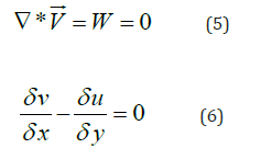
How to cite this article: Farhad Sakhaee. Finite Difference Method in Fluid Potential Function and Velocity Calculation . Trends Tech Sci Res. 2022; 5(4): 555670. DOI: 10.19080/TTSR.2022.05.555670
Abstract
There is no deterministic solution for many fluid problems but by applying analytical solutions many of them are approximated. In this study an implicit finite difference method presented which solves the potential function and further expanded to drive out the velocity components in 2D-space by applying a point-by-point swiping approach. The results showed the rotational behavior of both potential function as well as velocity components while encountering central obstacle.
Keywords: Implicit finite difference method; Fluid potential function; Velocity components.
Introduction
Finite difference method is a strong tool which has been developed by Euler in 1768 and extensively used in computational fluid dynamics problems. For instance, rate of transported particles in a river or coastal area depends on stream power and current direction. Stream power defined as shear stress multiplied by velocity. Hence velocity field calculations are essential element in derivation of sediment pattern in coastal areas to protect and sustainably manage coast structures such as breakwaters [1]. It can also be used in floodplain delineation as well as sediment velocity calculations. This study focused on a point-by-point implicit application to develop a MATLAB code which can derivative fluid velocity from fluid potential function.
Finite Difference Modeling
Finite difference method is a derivation of Taylor’s polynomial series expansion. The error in this method is defined as the difference between the approximation and exact analytical solution. It can be used in computational fluid dynamic modeling, heat transfer problems in both explicit and implicit forms. For instance, in explicit method, a forward difference in time and a second order central difference in the space (FTCS) approach may be applied and in its implicit form one can use a backward difference in time and second-order central difference in space (BTCS) to complete the simulation process [2-6]. Many applications in chemical engineering, fluid mechanics and geology involve interaction of particles and fluid which applies Navier-Stokes simulation by finite difference approach in a particle-laden flows [7, 8]. The goal of this study was to calculate the velocity components of U and V in x and y directions, respectively.
Materials and Methods
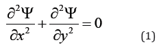
Potential function has been driven in a 20 × 20 meters box as in figure 1, including a central obstacle at the middle by an opening at each direction. Central box has a dimension of four meters. The potential function is defined by equation 1 below.
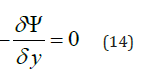
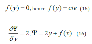
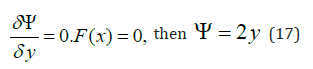
modelling
Conservation of mass and non-rotational-ideal fluid conditions have been applied to the model which are explained below in detail.
modelling
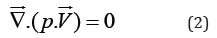
Applying conservation of mass in terms of this problem resulted in equation 2 as bellow [9-12].

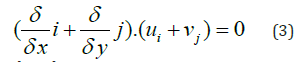
By expanding equation 2 we will have
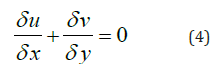
Finally, it reduced to.
Ideal-Non-Rotational-Fluid
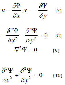
Velocity components of u and v presented below and, replaced in equation 6
Point-By-Point Method
In this method, every single point got its value from four adjacent neighbor points equation 11 showed this issue [13, 14].
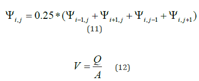
Velocity is equal to discharge over area; thus, velocity is equal to 2m/s for the unit area.
Discretization
To obtain an acceptable accuracy domain has been discretized. The entire domain consists of mesh size of 1m times 1m including 400 smaller boxes. Each one meter also has been divided into 6 segments (k=6) which finally resulted in 120 × 120 boxes. Figure 2(a, b) showed a schematic view of side segmentation [15, 16].
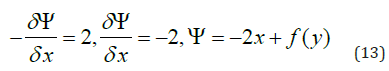
In equation 13 in velocity calculation, velocity in y direction, v is a constant. In terms of simplicity of calculations, considered to be zero.
Procedure
Considering the central internal box, fluid will encounter an obstacle at the center of bigger space. Considering potential function to be zero at the surface of internal box (Figure 3).


Calculations has been done through iterations for each of internal spaces until reaching a negligible amount of error which is presented by Epsilon =10-4.
Results
Case 1: Without central obstacle
Without having central obstacle line by line swiping provides the potential function for the entire area as presented in figure 4(a, b).
Case 2: With central obstacle
By considering small box at the center the potential function behavior and velocity distribution changed into two groups. One group moves from upper part of obstacle and the other one redirected toward beneath path, but both meets each other after the central box. Consequently, x and y components of the velocity can be driven out of potential function for each case which is provided in figure 5.


Conclusion
The novelty of this study is to find a finite difference numerical solution to approximate fluid potential function. Physical interpretation of the problem is a key component to understand the behavior of the fluid in such examples and converts the abstract problem an into a more comprehendible and pragmatic problem-solving tool. Ψ is the Potential function and as soon as the water reaches the central obstacle it starts rotating around to find its path towards the exit. This trend is observable within both potential function as well as velocity component path. Convergence and divergence of flow patterns could be observed both in the experimental visualization fluid dynamics lab as well as computational dynamic modeling CFDs [17].
Declaration of Conflict of Interests
The author declares that there is no conflict of interest. They have no known competing financial interests or personal relationships that could have appeared to influence the work reported in this paper.
MATLAB CODE
Case 1: Without central obstacle
clc
clear all
tic
k=6;
N=20*k+1;
Dx=20/(N-1);Dy=Dx;
psi=zeros(N);u=psi;v=u;
x=linspace(2,3,k+1);
y=linspace(17,18,k+1);
psi(N,2*k+1:3*k+1)=-2*x;
psi(2*k+1:3*k+1,N)=2*y;
v(N,2*k+1:3*k+1)=2;
u(2*k+1:3*k+1,N)=2;
error=1;temp=psi;
epsilon=1e-4;count=0;
while error>epsilon
for i=2:20*k
for j=2:20*k
psi(i,j)=0.25*(psi(i,j-1)+psi(i,j+1)+psi(i-1,j)+psi(i+1,j));
end
end
error=max(max(abs(temp-psi)));
temp=psi;
count=count+1;
end
for i=2:N-1
for j=2:N-1
u(i,j)=(psi(i-1,j)-psi(i+1,j))/2/Dy;
v(i,j)=-(psi(i,j+1)-psi(i,j-1))/2/Dx;
end
end
psi=flipud(psi);
u=flipud(u);
v=flipud(v);
x=linspace(0,20,N);
contour(x,x,u,10000)
xlabel('x(m)')
ylabel('y(m)')
title('velocity in x direction (m/s)')
figure (2)
contour(x,x,v,10000)
xlabel('x(m)')
ylabel('y(m)')
title('velocity in y direction (m/s)')
figure (3)
contour(x,x,psi,10000)
xlabel('x(m)')
ylabel('y(m)')
title('contour of \psi')
toc
Case 2: With central obstacle
clc
clear all
tic
k=6;
N=20*k+1;
Dx=20/(N-1);Dy=Dx;
psi=zeros(N);u=psi;v=u;
x=linspace(2,3,k+1);
y=linspace(17,18,k+1);
psi(N,2*k+1:3*k+1)=-2*x;
psi(2*k+1:3*k+1,N)=2*y;
v(N,2*k+1:3*k+1)=2;
u(2*k+1:3*k+1,N)=2;
error=1;temp=psi;
epsilon=1e-4;count=0;
while error>epsilon
for i=2:8*k
for j=2:20*k
psi(i,j)=0.25*(psi(i,j-1)+psi(i,j+1)+psi(i-1,j)+psi(i+1,j));
end
end
for i=8*k+1:12*k+1
for j=2:8*k
psi(i,j)=0.25*(psi(i,j-1)+psi(i,j+1)+psi(i-1,j)+psi(i+1,j));
end
for j=12*k+2:N-1
psi(i,j)=0.25*(psi(i,j-1)+psi(i,j+1)+psi(i-1,j)+psi(i+1,j));
end
end
for i=12*k+2:N-1
for j=2:20*k
psi(i,j)=0.25*(psi(i,j-1)+psi(i,j+1)+psi(i-1,j)+psi(i+1,j));
end
end
error=max(max(abs(temp-psi)));
temp=psi;
count=count+1;
end
for i=2:N-1
for j=2:N-1
u(i,j)=(psi(i-1,j)-psi(i+1,j))/2/Dy;
v(i,j)=-(psi(i,j+1)-psi(i,j-1))/2/Dx;
end
end
psi=flipud(psi);
u=flipud(u);
v=flipud(v);
x=linspace(0,20,N);
contour(x,x,u,10000)
xlabel('x(m)')
ylabel('y(m)')
title('velocity in x direction (m/s)')
figure (2)
contour(x,x,v,10000)
xlabel('x(m)')
ylabel('y(m)')
title('velocity in y direction (m/s)')
figure (3)
contour(x,x,psi,10000)
xlabel('x(m)')
ylabel('y(m)')
title('contour of \psi')
toc
References
- Sakhaee F, F Khalili (2021) Sediment pattern & rate of bathymetric changes due to construction of breakwater extension at Nowshahr port. Journal of Ocean Engineering and Science 6(1): 70-84.
- Lipnikov K, G Manzini, M Shashkov (2014) Mimetic finite difference method. Journal of Computational Physics 257: 1163-1227.
- Narasimhan T, P Witherspoon (1976) An integrated finite difference method for analyzing fluid flow in porous media. Water Resources Research 12(1): 57-64.
- Wu CH, BF Chen (2009) Sloshing waves and resonance modes of fluid in a 3D tank by a time-independent finite difference method. Ocean Engineering 36(6-7): 500-510.
- Chouet B (1986) Dynamics of a fluid‐driven crack in three dimensions by the finite difference method. Journal of Geophysical Research: Solid Earth 91(B14): 13967-13992.
- Yu B, Y Kawaguchi (2004) Direct numerical simulation of viscoelastic drag-reducing flow: a faithful finite difference method. Journal of Non-Newtonian Fluid Mechanics 116(2-3): 431-466.
- Höfler K, S Schwarzer (2006) Navier-Stokes simulation with constraint forces: Finite-difference method for particle-laden flows and complex geometries. Physical Review E 61(6): 7146.
- Colella P, MR Dorr, DD Wake (1999) A conservative finite difference method for the numerical solution of plasma fluid equations. Journal of Computational Physics 149(1): 168-193.
- Shen J, X Yang, Q Wang (2013) Mass and volume conservation in phase field models for binary fluids. Communications in Computational Physics 13(4): 1045-1065.
- Grinfeld P (2009) Exact nonlinear equations for fluid films and proper adaptations of conservation theorems from classical hydrodynamics. Journal of Geometry and Symmetry in Physics 16: 1-21.
- McCormack P (2012) Physical fluid dynamics. Elsevier, Netherlands.
- Kay JM, RM Nedderman, R Nedderman (1985) Fluid mechanics and transfer processes. CUP Archive. Pp: 602.
- E Oñate, S Idelsohn, OC Zienkiewicz, RL Taylor (1996) A finite point method in computational mechanics. Applications to convective transport and fluid flow. International journal for numerical methods in engineering 39(22): 3839-3866.
- Pletcher RH, JC Tannehill, D Anderson (2012) Computational fluid mechanics and heat transfer. CRC press, USA.
- Min T, JY Yoo, H Choi (2001) Effect of spatial discretization schemes on numerical solutions of viscoelastic fluid flows. Journal of non-newtonian fluid mechanics 100(1-3): 27-47.
- Dupret F, J Marchal, M Crochet (1985) On the consequence of discretization errors in the numerical calculation of viscoelastic flow. Journal of non-newtonian fluid mechanics 18(2): 173-186.
- J Galindo, A Tiseira, P Fajardo, R Navarro (2011) Coupling methodology of 1D finite difference and 3D finite volume CFD codes based on the Method of Characteristics. Mathematical and Computer Modelling 54(7-8): 1738-1746.


