


A GA-Based Accelerator for Solving Sparse Matrices
Khaled Salah*
Ain Shams University, Egypt
Submission: November 16, 2018; Published: December 18, 2018
*Corresponding author: Khaled Salah, Ain Shams University, Egypt.
How to cite this article: Khaled Salah. A GA-Based Accelerator for Solving Sparse Matrices. Robot Autom Eng J. 2018; 4(2): 555631. DOI: 10.19080/RAEJ.2018.04.555631
Abstract
This paper presents a novel hardware solution for solving sparse matrices using emulation technology. The proposed solution introduces a bio-inspired technique, which is Genetic Algorithm (GA) to solve the sparse system of linear equations (SLEs). The proposed solution can be used with any physical system that can be modeled as SLEs. Computations involved in Finite Element Method (FEM) consume too much time, which affects the final time-to-market value. Profiling shows that the most time-consuming part in the simulation process is the solver part which is responsible for solving the resultant SLEs generated from the FEM. The total number of equations may reach thousands or millions of linear equations. Hardware implementation of GA and making a good use of parallelism in implementing the architecture accelerate the time taken by the solver part. Solving the system by classical numerical methods, such as conjugate gradient (CG) implemented in software is performed sequentially, here the architecture allows the parallelism in performing GA operators, such as selection, crossover, and mutation. The parallelism in the proposed architecture is the superiority point which we rely on. The results show that our proposed method to solve the SLEs outperforms the classical CG software implementation on run time and number of equations.
Keywords: Matrix, Emulation, Genetic Algorithm, FPGA.
Introduction
The power harvesting from ambient vibrations can be stored to support wireless sensors which are applied for temperature and humidity measurement and machinery acceleration monitoring. Such vibration-based generators can automatically transform mechanical energy into electrical energy to supply the maintenance-free, wireless electronics. The piezoelectric effect is an effective method of electromechanical transduction. Cantilever-type piezoelectric generators with piezoelectric patches have recently received increasing attention over the past two decades [1].
Simulation of electromagnetic fields is growing in importance as a planning tool for high frequency systems. All available optimization opportunities can already be exploited in the design phase of, for example, an antenna or radar system, allowing for the performance of the final product to be maximized. The precise modeling of the relevant physical interactions in a simulation environment constitutes a large part of this optimization process and ensures that the developed system is optimally adapted to blend into its environment. The main objective of an electromagnetic (EM) Simulation Process is to find an approximate solution to Maxwell’s equations that satisfies given boundary conditions and a set of initial conditions. The key steps are:
A. Creation of the Physical Model: Drawing/Importing Layout Geometry, Assigning Materials, etc...
B. EM Simulation Setup: Defining Boundary Conditions, Ports, Simulation Settings, etc...
C. Perform the EM Simulation:
a. Discretizing the physical model into mesh cells and approximating the field/current using a local function (Expansion/Basis function)
b. Adjusting the function coefficients until the boundary conditions is satisfied
D. Post-processing: Calculating S-parameters, TDR Response, Antenna Far Field Patterns, etc.
The third step is the most important, as it depends on the type of solver used. There is a variety of numerical techniques for solving Maxwell’s equations and Partial Differential Equations (PDEs), in general. Most of these techniques result in SLEs that need to be solved simultaneously. A great part of the simulation time is consumed in solving these equations. As a result, Software-based electromagnetic solvers are often too slow.
Solving such problems may easily take traditional CPUs a couple of days, even months. An alternative is to build specific computer systems using ASICs, but this approach requires a long development period, and is inflexible and costly. GPUs provide a new approach and are based around a large number of simplified CPU-units. Unfortunately, GPUs are not suitable for problems that are data-intensive due to the long latency of memory. Based on the discussion above, HW facilities were used to accelerate these solvers [1].
There has been some related work to solve and accelerate solving sparse matrices. Steiblys [2] solves the SLEs using three different methods, for the hyper-power method the author solved a system of 200 equations, for the conjugate gradient method he ran different test cases with different sizes vary from 4704 equations to 525825 equations, and for the Monte Carlo method he solved a 200-equation system. The authors did not mention the run-time. Rashid & Crowcroft [3] presented a parallel Jacobi iterative algorithm for the steady-state solution of large Continuous Time Markov Chains (CTMCs). The parallel implementation was benchmarked using three widely used CTMCs case studies.
The steady-state solutions for large CTMCs were obtained, and it was shown that the steady-state probabilities for a Polling CTMC with approximately 1.25 billion states can be computed in less than 8 hours using 24 processors. Al Dahoud, et al. [4] has shown how genetic algorithms can be successfully applied to solve linear equations systems. They solved a system of two linear equations with a population size of seven chromosomes, although they did not state the runtime. Abiodun [5] introduced genetic algorithm as a method of solving SLEs. In a comparison between gaussian emulation and GA to solve the system, they showed that GA is more effective than conventional numeric al methods. They solved a system of four equations simultaneously. Also, the authors did not state the runtime and the number of solved equations is very small. Our key contributions of this paper compared to related work are as follows:
I. Solving large number of equations, which may reach thousands or millions of linear equations in less time than the time taken by the existing solutions, such as CG software approach.
II. Proposing a massively Parallel architecture of GA which outperforms the sequential software implementation.
The rest of paper is organized as follows. In section II, a brief background on technique we used, the system we solve and the technology we use are provided. The proposed architecture and the hardware implementation are presented in Section III. Test cases and results are explained in section IV. Conclusions are given in section V.
Background
In this section, the sparse SLEs is introduced, then the artificial technique used in solving the system, then the technology used in running and testing the proposed design.

Also, it can be written in a more compact vector-matrix form as:

This system can be one of three types based on m and n in
the previous equations. If m=n i.e. there are as many equations
as unknowns, then the system of equations is called exactly
determined. If m>n i.e. there are more unknowns than equations,
then the system of equations is called underdetermined. If m GA was invented by John Holland in the 1960s [7]. The
original goal was not to design algorithms to solve specific
problems, but rather to formally study the phenomenon
of adaptation as it occurs in nature and to develop ways
mimicking the adaptation, which might be imported into
computer systems. To solve a problem using GA, the algorithm
starts with a random initial population consists of number of
individuals each individual represents a possible solution to
the problem. Over iterations the algorithm creates a sequence
of new populations. At each iteration, the algorithm uses
the individuals of the current generation to create the new
individuals in the new generation. The new generation is
obtained by performing the following operations: a. Calculate fitness value of each individual from a predefined
fitness function. b. Scale the raw fitness values to convert them into
relative values can be more usable in the next step. c. Selection operator is responsible for selecting
parents based on their fitness values. The individuals with
high fitness have high probabilities to be passed to new
generation. d. Crossover operator is responsible for producing
offspring by combining the content of a pair of selected
parents. e. Mutation operator is responsible for making random
changes to a single crossover outcome offspring. f. Finally, the current population is replaced with the
mutation outcome offspring to be the new population. The algorithm continues in iterative manner till one of the
individuals reaches stopping criteria. Hardware emulation is becoming a popular solution
to runtime problems that afflict event-based software
simulators. It achieves execution speeds five to six orders
of magnitude faster than that delivered by RTL simulators
[8]. By 2005, only three players competed in the emulation
market: Cadence Design Systems, Mentor Graphics and EVE
(Emulation and Verification Engineering), each promoting
its own architecture. Today, hardware emulation is at the
foundation of every verification strategy, and it has become
a permanent fixture in SoC design. Embedded software is
forcing project teams to debug hardware and develop software
in parallel. With emulation, they now have the means to do it
fast, efficiently and cost effectively. New emulation solutions
are meeting the need and creating a new era for hardware and
embedded software designs [9]. Genetic algorithm
Hardware emulation
The Proposed Method
In this section, we will introduce the proposed parallel architecture and the hardware implementation details and platform we used to run code.
The proposed architecture
The proposed architecture shown in Figure 1, models a single iteration of the parallel design of classical GA with some modifications and optimization. This design consists of control unit, ALU, N instances of fitness module, N instances of selection module, N instances of crossover module, N instances of mutation module, diagonal elements of coefficient [A] matrix memory, non-zero non-diagonal elements of coefficient matrix [A] memory, right hand side [B] memory, N new and old population memories, fitness values memory, final solution memory, and fitness compare module. As the architecture models the classical GA, it starts with an initial population composed of N random individuals stored over N memories, each memory is a column vector of n elements. The first step is computing the fitness values of each individual this work is done over two sub-steps, starting with multiplying A matrix by individual then subtracting B vector from the multiplication resultant− where P is the ith individual. Since A matrix is a special sparse matrix, we do not need to store all elements, the diagonal elements and the non-zero non-diagonal elements are only stored.

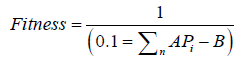
The control unit has the responsibility of deriving the addresses of the current elements to be sent to ALU and ALU do the arithmetic operations. The resultant is stored over N column vectors. The content of each vector is summed up in one register by accumulator sum module, the value of this register is sent to fitness module. Then fitness module calculates fitness value of each chromosome as:
After that we select the parents according to their fitness values by the roulette wheel selection operator. The control unit is responsible of enabling reading from the selected parents’ memories. The crossover module decides if the crossover will be performed or not according to random probability number and if yes where to crossover. The crossover is done by merging the content of selected parents’ memories to other new memories. The mutation module is similar to crossover module, though the mutation is done by changing only one specific element in the new memory. We need N new memories to represent the new population after crossover and mutation operators are done.
After doing all work and generating the new population, we added a step to the algorithm which compares the fitness of the old population to the fitness of the new population keeping the individual which has the higher fitness value. This step makes the algorithm converges faster to the final solution. The control unit is responsible of iterating this sequence till reaching stopping criteria and the halt signal is raised. The final solution is stored in a memory after raising halt signal.
Hardware implementation
The proposed solution can be used with any physical system that can be modeled as SLEs. Computations involved in FEM consume too much time, which affects the final timeto- market value. While the most time is consumed by the solver part which is responsible for solving the resultant SLEs generated from the FEM and the total number of equations may reach thousands or millions of linear equations. We headed to implement the solver part on hardware and using bio-inspired techniques, such as GA to accelerate solving the SLEs. The results show that our proposed solution is better than the software CG over runtime and number of equations.
Testing and results
The GA operation is tested by designing a Verilog testbench. The results of the proposed architecture for solving different equations as compared to the hardware implementation of the most famous conventional method conjugate gradient (CG) are shown in TABLE I. Compared to CG, the proposed architecture achieves better performance in terms of run time with max error of less than 2%. The number of used chromosomes is 200 Table 1.

Conclusion
The objective of this work is to adopt the GA-based accelerator to shorten the solving time of linear equations. We have implemented parallelism hardware architecture with central idea of GA genetic algorithm. Compared with the traditional CG algorithm, it outperforms by processing massive linear equations in runtime.
References
- Mohamed K, AbdelSalam M (2017) Solving Sparse Matrices: a Comparative Analysis between FPGA and GPU.
- Steiblys L (2014) Iterative Methods for Solving Systems of Linear Equations: Hyperpower, Conjugate Gradient and Monte Carlo Methods, Manchester. University of Manchester Faculty of Engineering and Physical Sciences, Manchester, England, p. 1-61.
- Rashid M, Crowcroft J (2005) Parallel iterative solution method for large sparse linear equation systems. University of Cambridge, Computer Laboratory, Cambridge, England, p. 1-22.
- Al Dahoud A, Ibrahiem MMEl Emary, Mona Abd El-Kareem M (2009) Application of Genetic Algorithm in Solving Linear Equation Systems. MASAUM Journal of Basic and Applied Science 1(2): 179-185.
- Abiodun I (2011) The Effectiveness of Genetic Algorithm in Solving Simultaneous Equations. International Journal of Computer App14(8): 2011.
- Axler S (1995) Linear Algebra Done Right. Springer International Publishing, Cham, Switzerland.
- Mitchell M (1998) An Introduction to Genetic Algorithms. Cambridge, MA, USA: MIT Press, England.
- Rizzatti DL (2014) Electronic Design.
- Rizzatti DL (2015) Hardware Emulation: Three Decades of Evolution- Part III. verification horizone 11(1): 1-4.


