Case Report

Producing Contiguous Data in Marine Environment: A Gaussian-Montecarlo Methodology

Giuseppe MR Manzella¹*, Marco Gambetta² and Antonio Novellino¹

¹ETT SpA, Genova, Italy

²CGG Marine Engineering, Italy

Submission: July 22, 2018; Published: September 04, 2018

*Correspondence author: Giuseppe MR Manzella, ETT SpA, Genoa, Italy.

How to cite this article: Giuseppe M M, Marco G, Antonio N. Producing Contiguous Data in Marine Environment: A Gaussian-Montecarlo Methodology. Oceanogr Fish Open Access J. 2018; 8(3): 555736. DOI:10.19080/OFOAJ.2018.08.555736

Abstract

Marine environment is strongly undersampled. Spatial data have an inhomogeneous spatial as well as temporal distributions and the production of tri-dimesional maps are still posing problems of interpretation of their results. This paper is proposing a mapping methodology based on Gaussian- Montecarlo approach that create additional synthetic data having the environmental characteristics of their neighborough data profiles. With respect to other methodologies, the one presented in this paper is not filtering out the small-dimension characteristics.

Keywords: Marine environment; EMODnet physics; Spatial interpolation

Introduction

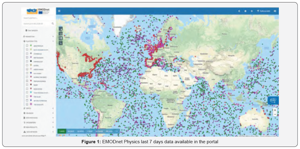
The marine environment is under different anthropogenic pressures, such as coastal developments, offshore activities, overfishing. To support a sustainable use of our seas and oceans, the European Commission produced a directive with some methodological standards to be adopted by EU Member States to assure a good environmental status of marine waters. Directive and standards were accompanied by an important initiative called ‘The European Marine Observation and Data Network’ (EMODnet) having the aim to provide information to many different users. EMODnet is composed by seven thematic portals, among which Physics is providing data on: sea water temperature, sea water salinity, sea water currents, sea level, waves and winds (speed & direction), water clarity (light attenuation), atmospheric parameters at sea level, underwater noise, river data. A snapshot of last 7 days data coverage from different platforms accessible throuth the EMODnet Physics Portal is provided in Figure 1 (www.emodnet-physics.eu).

One of the challenges is to produce contiguous data over a maritime basin from fragmented, inhomogeneous data. There are many methodologies that are using to interpolate in situ data in order to represent a physical state in a particular time period. Some of them are based on statistics, others are based on some the knowledge of phenomenological scales, finally there are methodologies that are taking into considerations the dynamics of the marine circulation.

Observations always have inaccuracies. In general it is supposed that observations are the sum of many independent processes and have a normal (or Gaussian) distribution (or nearly normal). Statistic theory provides powerful methods for obtaining the most reliable possible information from a set of observations. The principles behind these methods can be derived from the principle of maximum likelihood, if the errors follow the Gauss distribution. In general, for underlying statistical model, the method of maximum likelihood is used to select set of values of model parameters that maximizes the likelihood function. This maximizes the “agreement” of the selected model with the observed data and maximizes the probability of the observed data under the resulting distribution.

Additionally, to the observational inaccuracies, in oceanography there is another problem related to the uneven temporal and spatial coverage of the observations. Normally, maps of environmental characteristics are obtained with methodologies (e.g. kriging, optimal interpolation) that filter out the high-frequency and smallscale phenomena. A particular methodology can be applied in case of synoptic data (i.e. data collected within a short period time) in order to avoid those filtering effects.

Case Reports

Synthetic oversampling

The ocean is dramatically under sampled and this is the main problem that pushed for the development of interpolation techniques. A way to add ‘stations’ in a particular area can be obtained using a Montecarlo method that is derived from the Gaussian interpolation. An exercise has been done by using an initial dataset composed by a 98 CTD casts of temperature / salinity vertical profiles, collected in February 19 - 22, 2007 over an area of about 90x100km in the northern Adriatic Sea by CNR-ISMAR from Bologna and the Emilia-Romagna regional environmental agency – Daphne (Figure 2 - left).

The algorithm finds, within the area, a number of randomly simulated stations and for each of them computes temperature and salinity seawater vertical profiles.

Definition of randomly placed stations

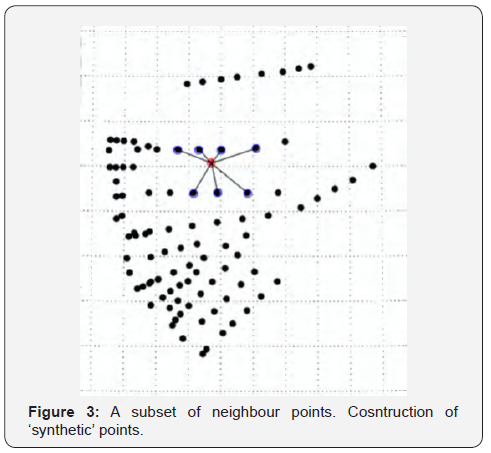
In open sea, the sampling strategy is based on the internal radius of deformation, i.e. a distance that is considering the characteristic scales of phenomena. In coastal and shelf areas, this concept cannot be applied since the phenomena scales are biased by the bathymetry and coastline effects and different criteria must be defined. The simulation locations, which are the points where T/S profiles are calculated (Figure 2 right), are randomly defined with constraints based on the nearest neighbor distance and the local sea depth. The algorithm uses a recursive logical structure to find a suitable location that assures both randomness and homogeneity inside to pre-defined depth ranges which correspond to adjacent polygons on the sea surface. In detail, the iterative procedure is the following one (Figure 3):

I. The original bathymetric data are interpolated to have a new bathymetric chart with a resolution of 50m.

II. The area is divided in strips defined by the bathymetries of 0-7, 7-15, 15-35 and greater than 35 metres.

III. For each of these strips the number of stations to be simulated and the minimum distance between stations are defined.

The randomly generated positions respecting the above conditions are accepted as part of the ‘synthetic’ oversampling. In this way, the goal of having a random sampling with a bathymetric controlled wavelength is achieved. The new bathymetry with 50m resolution, defined in the step 1 of the procedure, is reconstructed from the metadata, contained in the initial dataset, using bi-dimensional cubic interpolation. In total, 458 “synthetic” stations have been randomly placed in the area.

For each of the previously simulated locations the algorithm selects a number of neighbour stations among the sampled dataset. These stations are selected accordingly to a search radius empirically defined hereafter:

sR = -1,758z 2 + 172,4z + 139,0

where sR is the search radius (in metres) and z (in metres) is the sea depth at the i-th simulated location.

Figure 3 shows the initial dataset (black filled dots) and a subset of neighbour points (black dots outlined with blue), selected by the algorithm during the simulation of temperature and salinity profile at a specific location (red dot).

Results

Simulation of temperature

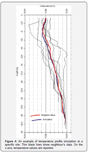
For each simulated location, a certain number of neighbours observed profiles are selected and temperature values at each depth is evaluated by a random value within the data envelop. Considering

Where, is the set of the temperature values sampled at a specific depth z in all n neighbor stations and is the mean averaged temperature profile (see Figure 4):

Where, is the weight of the “i-th” neighbor station data defined as an inverse function of the distance between the station itself and the current simulation station (see Figures 3 & 4). The weighted variance is defined in the same way.

Since the observed temperatures show a near normal distribution, a set, of simulated temperature values is randomly generated with normal distribution so as to respect the following:

Where being a positive real number and k being a user defined value as a measure of overall variability allowed to the simulation procedure. High k values give quite noisy simulations. Then, a third-degree polynomial spline is applied to smooth the simulated temperature profile.

Simulation of salinity

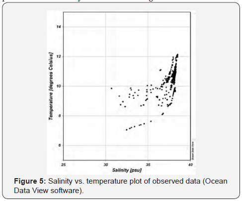
For the calculation of salinity a third degree polynomial spline is calculated from T/S diagrams (Figure 5) of all sampled data. Using this polynomial function a corresponding salinity vertical profile is calculated from any temperature value. This method assures the stability of the density profiles in the water column.

Temperature Maps

Map of temperature observed at surface is shown in Figure 6, the temperature map at surface obtained from simulated over-sampling is shown in Figure 7. Maps have been obtained applying a minimum curvature algorithm. Grid size in figures is 1000m; contour interval is equal to 0.25 °C. The original data (Figure 6) shows a general north-south alignment of isotherms with few meanders. The coastal area is characterised by the presence or relatively cold water coming from rivers.

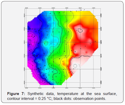
The shelf water is warmer and is divided from the coastal water by significant thermal gradients. Figure 6 shows that three different water masses could be defined: coastal, shelf and transitional water, comprised between 10.75 and 11.75 °C. The general behaviour of original data is maintained in the “synthetic” map, but more complex features are created by the over-sampling. The three water masses are occupying the same areas and the thermal gradient dividing them is maintained (Figure 7). However, meanders are much more pronounced with respect to the smoother behaviour of the original data. In general, short wave-lengths components are added to the original data.

Salinity maps

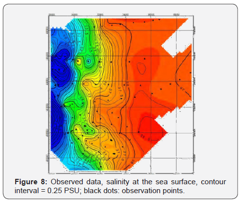
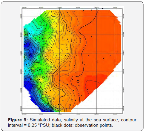
The “synthetic” salinity is calculated from T-S diagram as previously explained. Figure 8 & 9 show respectively observed and estimated data. The salinity field shows the presence of tree water masses. The separation of coastal waters from the transitional layer is characterised by a significant haline gradient. The shelf water is spatially homogeneous.

In general, the “synthetic” salinity present meanders at the limit of the coastal waters and a minor spatial homogeneity on the shelf area [1-4].

Conclusion

One dimensional interpolation, although presenting problems related to the addition of errors, can provide results that can be quite easily interpretable without controversies. Very different is the 2D, 3D or even 4D interpolation. Existing techniques can provide different maps. A Gaussian – Montecarlo method has been applied to a particular case, but also in this case the production of maps is quite complex. The conclusion is that the different methods could be applied, but a comparison between different results can help the interpretation of phenomena shown in maps.

Acknowledgment

This work was performed within the framework of the DGMARE EMODnet-Physics project. Authors Manzella was employed by ETT SrL. All authors declare no competing interests.

References

1. Crochiere RE, Rabiner LR (1983) Multivariate Digital Signal Processing. Englewood Cliffs, Prentice Hall, New Jersey, USA.
2. Young HD (1962) Statistical Treatment of Experimental Data. McGraw- Hill, New York, USA, 7(1): 72.
3. Wahba G (1990) Spline Models for Observational Data 59. SIAM 161.
4. Williams CKI (1998) Prediction with Gaussian Processes: From Linear Regression to Linear Prediction and Beyond. Learning in Graphical Models 599-621.