Oceanography & Fisheries Open access Journal (OFOAJ)

Review Article

Water Quality Modelling For Ocean Engineering m Projects - A Review

Manivanan R*

Central Water and Power Research Station, India

Submission: March 01, 2017; Published: July 06, 2017

*Corresponding author: Manivanan R, Central Water and Power Research Station, Khadakwasla RS, Pune-411 024, Maharastra State, India, Email: vananrmani@rediffmail.com

How to cite this article: Manivanan R. Water Quality Modelling For Ocean Engineering Projects - A Review. Ocean & fish Open Access J. 2017; 3(4): 555617. DOI:10.19080/OFOAJ.2017.03.555617

Introduction

Water plays an important role in our daily life and without it no life on the earth. Most activities in our life depend on water such as drinking, agriculture, a medium of transportation and many more. In fact, many great civilizations have started near to the source of water whether river, lake, coastal etc. such as Mesopotamia, Egypt, and many more.

Water quality models can be effective tools to simulate and predict pollutant transport in coastal water environment, which can contribute to saving the cost of labours and materials for a large number of industrial development in the coastal region. Therefore, water quality models become an important tool to identify water pollution and the final fate and behaviours of pollutants in coastal environment. These developmental projects such as nuclear power plants, desalination plants, ports and harbours construction projects can bring serious effects on coastal environment after enforcement. Therefore, these environmental impacts have to be analysed, simulated, predicted, and assessed using mathematical and numerical models before these construction projects are implemented. These modeling results under different pollution scenarios using water quality models are very important components of marine Environmental Impact Assessment. Moreover, they are also the important basis for environmental management decisions. With the development of model theory and the fast- updating computer technology more and more water quality models have been developed with various model algorithms. Up to date, tens of types of water quality models including hundreds of model software have been developed and applied for different topography, water bodies, and pollutants at different space and time scales.

Development of Water Quality Models

Water quality models have undergone a long period of development since Streeter & Phelps [1] built the first water quality model (S-P model) to control river pollution in Ohio state of the US [1]. Water quality models have made a big progress from single factor of water quality to multifactors of water quality, from steady-state model to dynamic model, from point source model to the coupling model of point and nonpoint sources, and from zero-dimensional mode to one-dimensional, two-dimensional, and three-dimensional models. More than 100 water quality models have been developed up to now. Cao & Zhang [2] classified these models based on water body types, model-establishing methods, water quality coefficient, water quality components, model property, spatial dimension, and reaction kinetics. However, each water quality model has its own constraint conditions [3]. Therefore, water quality models still need to be further studied to overcome the shortcomings of these current models.

The primary stage (1925-1965)

Water quality of water bodies has been paid much more attention during 1925 and 1965. The water quality models focused on the interactions among different components of water quality systems as affected by living and industrial point source pollution [4]. Like hydrodynamic transmission, sediment oxygen demand and algal photosynthesis and respiration were considered as external inputs, whereas the nonpoint source pollution was just taken into account as the background load [5].

The simple BOD-DO bilinear system model was developed and achieved a success in water quality prediction, and the onedimensional model was applied to solve pollution issues in rivers and estuaries [3]. After that, most researchers and scientists modified and further developed the Streeter-Phelps models (S-P models). For example, Thomas Jr [6] reported that oxygen consumption due to sediment deposition and flocculation processes. Connor O [7] divided BOD parameter into carbonized BOD and nitrified BOD and added the effects of dispersion based on the equation. Dobbins WE [8] added two coefficients, including the changing rate of BOD caused by sediment release and surface runoff as well as the changing rate of DO controlled by algal photosynthesis and respiration, to Thomas’s model.

The improving stage (1950-1975)

From 1965 to 1975, water quality models were classified as six linear systems and made a rapid progress based on further studies on multidimensional coefficient estimation of BOD-DO models. The one-dimensional model was updated to a two-dimensional models which were applied to water quality simulation of lakes and gulfs [9]. Nonlinear system models were developed during the period from 1970 to 1975 [10]. These models included the N and P cycling system, phytoplankton and zooplankton system and focused on the relationships between biological growing rate and nutrients, sunlight and temperature, and phytoplankton and the growing rate of zooplankton [5].

After 1975, the number of state variables in the models increased greatly, and the three-dimensional models were developed at this stage, and the hydrodynamic mode and the influences of sediments were introduced to water quality models [11]. The typical models including QUAL models, MIKE11 model, and WASP models were developed and used at this stage.

The advanced stage (after 1975)

Nonpoint source pollution has been reduced due to strong control in developed countries. Although nutrients and toxic chemical materials depositing to water surface have been included in model framework, these materials not only deposited directly on water surface but also they can be deposited on the land surface of a water body and sequentially transferred to water body [12]. Among the previously mentioned water quality models, these models including the Streeter-Phelps model, QUASAR model, QUAL model, WASP model, CE-QUAL-W 2 model, HEC-RAS model, MIKE model, and EFDC model were widely applied worldwide.

MIKE21 Dynamic Modelling tool Eco La

Dynamic ecological modelling tool is the basis for an ecosystem approach to environmental management. It allows quantitative, dynamic descriptions of water quality in the short or long term and includes nutrient dynamics, plankton, eelgrass, macroalgae and benthic fauna. The different standard ECO Lab models are developed and optimised to address specific environmental challenges. These include including varying climatic conditions and varying complexities from simple interactions to complex ecosystem models.

ECO Lab is the preferred solution for assessing factors such as:

Effects of nutrient loadings on the status of the aquatic environment
Strategies for wastewater treatment (nutrients and bacteria)
Causes and impacts of oxygen depletion events
Effects of cooling water discharges
Environmental impacts of constructing large infrastructures like harbours, bridges or tunnels
Impact of dredging on primary production and growth of benthic vegetation & mussels
Environmental consequences of developing new urban and industrial areas
Efficiency of action plans related to nutrient reductions and long term effects of reduction scenarios
Risks in connection with algal blooms
Site selection, optimisation of production and Environmental Impact Assessments (EIAs) in connection with aquaculture production.

With ECO Lab is a complete numerical laboratory for water quality and ecological modeling. It can simply define the process using standard templates as a basis. It enables to transform any aquatic ecosystem into a reliable numerical model for accurate predictions. ECO Lab uses a so-called ECO Lab object to perform the ECO Lab calculations. The ECO Lab object is generic and shared with a number of different hydrodynamic flow model systems. It consists of an interpreter that first translates the equation expressions in the ECO Lab template to lists of instructions that enables the object to evaluate all the expressions in the template. During simulation the model system integrates one time step by simulating the transport of advective state variables based on hydrodynamics. Initial concentrations or updated AD concentrations, coefficients/constants and updated forcing functions are loaded into the ECO Lab object and then the ECO Lab object evaluates all the expressions, integrates one time step, and returns updated concentration values to the general flow model system that advances one time step. An illustration of the data flow is shown in Figure 1.

MIKE21 ECOLAB Software

MIKE21 water quality simple (DO and BOD)

The main reason for modeling the dissolved oxygen concentration is to ensure that it is above acceptable levels for biota in the area under consideration. Oxygen in the aquatic environment is produced by photosynthesis of algae and plants and consumed by respiration of plants, animals and bacteria, Biological Oxygen Demand (BOD) degradation, sediment oxygen demand and oxidation of nitrogen compounds. In addition, dissolved oxygen is re-aerated through interchange with the atmosphere.The carbonaceous BOD is an expression of the water’s organic matter content. That is to say the biodegradable part of the organic matter which gives rise to oxygen consumption. The organic matter content is measured by registering the oxygen consumed during the degradation for a period of 5 days.

MIKE21 water quality with nutrients (nitrates, phosphates & ammonia)

The nutrients considered are the inorganic forms of nitrogen and phosphorus. The nitrogen cycle starts with an assimilation of free nitrogen from the atmosphere (e.g. blue green algae) or uptake by algae and plants of ammonia from the water. Degradation of dead organic matter leads to a release of the organic bound nitrogen in the form of ammonia. The degrading bacteria, however, utilize some of the nitrogen for their own growth. The rest of the ammonia released by ammonification or discharged from pollution

MIKE21 water quality simple including temperature and salinity

It simulates water quality parameters such as DO, BOD, with temperature and salinity concentration in the water ecosystem. This template used for investigation of pollution levels in the water ecosystem with temperature and salinity. It can be applied to modeling of intake/ outfall studies for nuclear, thermal and other power plants, reverse osmosis plants and desalination plants.

Modeling Techniques

For studies, mathematical model MIKE3 HD (DHI 2010) was used for simulation of hydrodynamics in the proposed area. The MIKE3 HD model was developed by Danish Hydraulics Institute (DHI), Denmark, and is widely used commercial software. Brief description of this model is given below.

The hydrodynamic model (MIKE21 HD)

The hydrodynamic model MIKE 21 -HD (DHI, 2010) was used for simulation of water levels and flows in coastal areas.

X-Direction

Y-Direction

Where,

Fluid acceleration
Horizontal gradients in the velocity,
Coriolis acceleration,
Acceleration from sea surface elevation,
Pressure gradient term,
Acceleration from buoyancy effects,
Imbalance of horizontal Reynolds stresses,
Vertical stresses from the Bousinesq approximation and
Acceleration from discharges

It simulates unsteady two-dimensional flows in coastal area and is based on the following non-linear vertically integrated 2-D equations of conservation of mass and momentum.

The model MIKE21 ECOLAB

The module is mostly used for modelling water quality as part of an Environmental Impact Assessment (EIA) of different human activities of estuary, creek and open ocean area with MIKE21,MIKE3, MIKE11 hydrodynamics. The strength of this tool is the easy modification and implementation of mathematical descriptions of ecosystems into the hydrodynamic software. The 2D depth-averaged transport equation for a non-conservative pollutant iis given as:

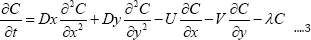
where Dx , Dy are the dispersion coefficients in x and y direction; U, V are the depth mean velocities in the x and y directions, respectively (m/sec); λ is the decay coefficient (s-1). This equation is numerically solved by an explicit finite difference scheme using MIKE21. The model outputs are evaluated using the performance criteria described in the next section.

Results

As the water quality plumes dispersed (Figure 2) shore attached on northward and southward directions and offshore region for existing outfall and along with proposed port, the plumes always towards offshore region and northward direction with minimum concentration. Hence, may not be observed any impact on coastline and proposed port region.

Water quality modelling using CORMIX system

The Cornell Mixing Zone Expert System (CORMIX) consists of a series of software subsystems for the analysis, prediction, and design of aqueous discharges into watercourses, with emphasis on the geometry and dilution characteristics of the initial mixing zone, including the evaluation of regulatory requirements. CORMIX1 deals with buoyant submerged single port discharges into flowing unstratified or stratified water environments. It includes the limiting cases of non-buoyant limiting cases. CORMIX3 deals with buoyant surface discharges into similar environments.

Reverse Osmosis Plant draws saline water from sea intake and converts it into potable water and discharges brine water at out fall as effluent. Mathematical model studies were carried out for dispersion of brine water with salinity of 63ppt from a Reverse Osmosis (RO) plant into coastal waters at north Chennai.

Studies were carried out to determine suitable locations of intake and outfall system for RO Plant such that recirculation of brine water is minimum (Figure 3). An Expert System called CORMIX II was used and studies were conducted for three alternatives namely alternative I which is 1000m distance from shoreline, alternative II is assumed 750m distance from shoreline and alternative III is 500m from shoreline.

The results depicted for alternatives I,II, the plume away from the intake and the possibility of recirculation of brine water is not observed. However there is a possibility of recirculation of brine water with 0.1ppt salinity in alternative-III. Hence, the alternative I and II are found suitable for the dispersal of brine water with vertical jet from a port diameter of 0.15m.

The alternative-I is expensive compared to alternative-II as it is 250m away from alternative-II. The study indicated that higher velocity and larger port diameter helps in enhancing dispersion rate and hence adverse effects on marine environment could be minimised [13].

Conclusion

The purpose of this lecture is to be explored possibilities of water quality modelling in the coastal region. Environmental analysts require estimates of water pollution levels and expected dispersion/transport patterns following intentional or accidental incidences and industrial waste releases to coastal environments. Water quality modelling assists in assessing potential impacts to human/environmental health and government operations by providing predictive estimates of pollutant concentration, speed and direction of travel. The water quality modelling is a useful tool for coastal engineering projects [14-16].

References

- Streeter HW, Phelps EB (1925) A Study of the Pollution and Natural Purification of the Ohio River. US Dept of Health, Edu and Welfare.
- Cao XJ, Zhang H (2006) Commentary on study of surface water quality model. Jr of Water Resources and Arch Eng 4(4): 18-21.
- Burn DH, McBean EA (1985) Optimization modeling of water quality in an uncertain environment. Water Resources Research21(7): 934-940.
- Wang JQ, Zhong Z, Wu J (2004) Steam water quality models and its development trend. Jr of Anhui Normal Univ 27(3): 243-247.
- Riffat R (2012) Fundamentals of Wastewater Treatment and Engineering. CRC Press, Boca Raton, Florida, USA.
- Thomas HA (1948) The pollution load capacity of streams. Water Sewage Works 95(11): 409-413.
- Connor DJO (1967) The temporal and spatial distribution of dissolved oxygen in streams. Water Reso Res 3(1): 65-79.
- Dobbins WE (1964) BOD and oxygen relationships in streams. Sanitary Eng Division, Amer Soc of Civil Engineers 90(3): 53-78.
- Gough DI (1969) Incremental stress under a two-dimensional artificial lake. Canadian Journal of Earth Sciences 6(5): 1067-1075.
- Yih SM, Davidson B (1975) Identification in nonlinear, distributed parameter water quality models. Water Reso Res 11(5): 693-704.
- Wolanski E, Mazda Y, Ridd P (1992) Mangrove hydrodynamics. Coastal and Estuarine Studies 41: 43-62.
- 1Esterby SR (1996) Review of methods for the detection and est. of trends with emphasis on water quality application. Hydro Processes 10(2): 127-149.
- Manivanan R, Renganath LR, Kanetkar CN (2006) Mixing zone simulation of brine water and solid dispersion performance in the coastal environment using mathematical models. APD IAHR Intl Conf IIT, Chennai, India.
- Manivanan R, Jha SN, Kudale MD (2014) Locating the intake and outfall structures of coastal plants through thermal/salinity dispersion studies. Intl Jr of Earth Sciences and Engineering 7(2): 439-446.
- Danish Hydraulic Institute (2010) MIKE21: Hydrodynamic Module, User Guide and Ref Man Horsholm. DHI, Denmark.
- Danish Hydraulic Institute (2010) MIKE 21: Eutrophication Module, User Guide and Reference Manual Release 2.7 Horsholm. DHI, Denmark.