Mini Review

The Burr II-R{Y} Family of Distributions

Clement Boateng Ampadu*

Department of Biostatistics, USA

Submission: October 24, 2019; Published: November 20, 2019

*Corresponding author: Clement Boateng Ampadu, Department of Biostatistics, USA

How to cite this article: Clement Boateng Ampadu. The Burr II-R{Y} Family of Distributions. JOJ Wildl Biodivers. 2019: 1(5): 555575 . DOI: 10.19080/JOJWB.2019.01.555575

Abstract

The Burr system of distributions [1] arise from a differential equation with solution

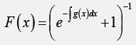
where g(x) is a function whose integrals are such that F(x) increases from 0 to 1 on the interval −∞ < x < ∞. Inspired by the T − R {Y} framework of creating probability distributions [2], this paper assumes T is a Burr II random variable, to introduce also-called Burr II-R{Y} family of distributions. A member of this family is shown to be a good fit to the precipitation data [3]. Finally, as this article is introductory in nature, the reader is asked to further investigate some properties and applications of this new class of statistical distributions.

Keywords: T-R{Y} family of distributions; Burr system of distributions; Precipitation data

Contents

a) Introduction and the New Family

b) Practical Illustration

c) Concluding Remarks and Further Recommendations

Introduction and the new family

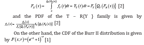
Let T, R, Y be random variables with CDF’s

corresponding quantile functions be denoted by QT (p), QR(p), and QY (p), respectively. Also, if the densities exist, let the corresponding PDF’s be denoted by ()()(),, f,TRYfxfxandxrespectively. Following this notation, the CDF of the T − R{Y } family is given by

On the other hand, the CDF of the Burr II distribution is given

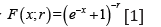
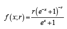
where < x<,−∞∞By differentiation, the PDF of the Burr II distribution is given by

From the CDF of the T − R {Y} family of distributions we have the following

Proposition 1.1. The CDF of the Burr II-R{Y} family of distributions is given by

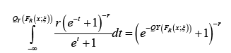
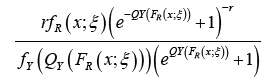
where the random variable Y has quantile QY , r > 0, and the random variable R has CDF FR. The parameter space of ξ and x depends on the chosen baseline distribution of the random variable R.by differentiating the CDF in the previous Proposition, we have the following.

Proposition 1.2. The PDF of the Burr II-R{Y} family of distributions is given by

where the random variable Y has quantile QY and PDF fY , r > 0, and the random variable R has CDF FR and PDF fR. The parameter space of ξ and x depends on the chosen baseline distribution of the random variable R The rest of this paper is organized as follows. In section 2, we illustrate the new family. The last section is devoted to the conclusions and some further recommendations (Figure 1).

Practical illustration

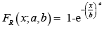
We assume R is a Weibull random variable with the following CDF

for x, a, b > 0. We assume Y is standard extreme value, so that

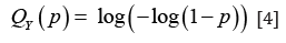
for 0 < p < 1. Now from Proposition 1.1, we have the following

Corollary 2.1. The CDF of the Burr II-Weibull {Standard Extreme Value} distribution is given by

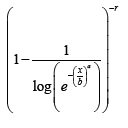
where x, a, b, r > 0

Notation 2.2. We write c  BIIWSEV (a, b, r), if C is a Bur IIWeibull {Standard Extreme Value} random variable.

Concluding Remarks and Further Recommendations

In this paper we introduced a so-called Burr II-R{Y} family of distributions and showed a member of this class of distributions is a good fit to the precipitation data [3]. As this paper is introductory in nature; we ask the reader to further explore some properties and applications of this new class of distributions.

References

1. Burr IW (1942) Cumulative frequency functions. Annals of Mathematical Statistics 13: 215-232.
2. Aljarrah (2014) On generating T-X family of distributions using quantile functions Journal of Statistical Distributions and Applications 1: 2.
3. Suleman Nasiru, Peter N, Mwita, Oscar Ngesa (2018) Discussion on Generalized Modified Inverse Rayleigh, Appl Math Inf Sci 12(1): 113-124.
4. Ayman Alzaatreh, Carl Lee, Felix Famoye (2014) T-normal family of distributions: a new approach to generalize the normal distribution, Journal of Statistical Distributions and Applications 1: 16.