


Sample Summary
Small-sample comparisons of binomial proportions often rely on Fisher’s exact test, which can be overly conservative and underpowered. We introduce a perturbation testing framework that generates exact tests by perturbing outcomes, with two variants: with replacement (WR) and without replacement (WOR). The WR test maintains nominal Type I error while achieving higher power than Fisher’s, Barnard’s, and Boschloo’s tests, and it extends naturally to multiple groups, outperforming the Freeman-Halton test. Implementable in just a few lines of R code, the WR perturbation test offers a fast, practical, and more powerful alternative to traditional exact methods.
Abstract
Small sample comparisons of binomial proportions are common in early phase clinical trials, laboratory studies, and rare event investigations. The standard test, Fisher’s exact, often lacks power due to conservative Type I error control. Alternatives like Barnard’s and Boschloo’s tests offer less conservative error control and greater power. We present a unified perturbation testing framework for generating exact tests by perturbing the discrete outcome variable, yielding two variants: with replacement (WR) and without replacement (WOR). For the null hypothesis H0: π1=π2, WR controls Type I error at the nominal level while providing uniformly higher power than existing methods. The approach extends naturally to g independent groups, where WR outperforms the Freeman-Halton exact test. Easily implemented in a few lines of R code and executing in seconds, the WR perturbation test offers a practical, more powerful alternative to traditional exact tests.
Keywords:Perturbation Test; Exact Inference; Small Sample Power; Randomization Test; Monte-Carlo Resampling
Introduction
Consider a randomized trial where subjects are assigned to one of two treatments, T1 or T2, using a standard parallel design. The primary outcome is binary, coded as 0 or 1. Suppose there are j = 1, 2, . . , n subjects, where subject j would have response x1j under treatment T1 and response x2j under treatment T2. The individual treatment effect for subject j is defined as x1j-x2j. However, in practice, only one of these two potential outcomes is observed for each subject due to random assignment.
Following the principles of randomization inference as outlined by Rosenbaum [1], and focusing on the binary outcome setting, assume that out of n=n1+n2 total subjects, n1 are randomly assigned to receive treatment T1 and n2 to receive treatment T2.
There is  possible treatment assignments, each equally likely with probability 1/m.
Let Ij=1 if subject j is assigned to treatment T1 and Ij=0 if assigned to T2. In randomization theory, the only source of randomness is this treatment assignment vector I= (I1, I2, . . ., In), where typically P (Ij = 1) =θ for j = 1, 2, . . ., n. The observed outcome for subject j is then given by the random variable  . This formulation enables the construction of the randomization distribution by enumerating all m possible assignments.
In the context of comparing binary outcomes between the two groups, we are interested in testing whether
 differs from
 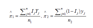 .
.
The corresponding estimators are:

In a one-sided testing scenario, we may test H0: π1=π2 versus H1: π1>π2 (or similarly H1: π1<π2). Define the observed test statistic as . For each of the m permutations, compute the corresponding test statistic
 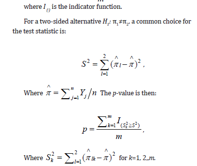 , for k = 1, 2, . . ., m. The exact p-value is then given by:

where I (·) is the indicator function.
For a two-sided alternative H1: π1≠π2 , a common choice for the test statistic is:
Where 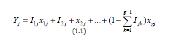 The p-value is then:

Where 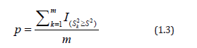 for k=1, 2,,m.
Since enumerating all possible treatment assignments is often computationally infeasible for large sample sizes, Monte Carlo approximations offer a practical alternative. Specifically, by randomly selecting B treatment assignments, the p-value can be estimated as:

for the alternative hypothesis H1: π1>π2, with analogous expressions for other alternatives. This method enables feasible inference under the randomization framework.
The randomization test corresponds to sampling without replacement from the set of all possible assignments. In addition, we will explore a bootstrap-like approach that samples with replacement from the observed outcomes Y. The Monte Carlo approximation to the p-value in this case follows the same logic as that used in the randomization test.
Practically, when comparing two treatments with a binary outcome, the observed data can be summarized in a 2×2 contingency table. In this setting, the p-values obtained through a randomization test is equivalent to those derived from Fisher’s exact test. Fisher’s exact test, introduced by R. A. Fisher in the 1930s [2], was specifically designed to analyze small 2×2 contingency tables. The test is rooted in conditional probability, famously illustrated by the” Lady Tasting Tea” experiment. The test is based on calculating the exact probability of observing a table as extreme as the one obtained, assuming the null hypothesis and conditioning on fixed row and column margins. This approach leads to the hypergeometric distribution as the basis for inference. Fisher’s ex- act test is widely used in biomedical and clinical research, especially where small sample sizes make large-sample approximations unreliable. There are several test statistics that are one-to-one that can be utilized using this approach that generate identical p-values [3].
However, Fisher’s test has some important limitations. It assumes fixed marginal totals, a condition that may not reflect many real-world randomization scenarios, such as those described previously where only the treatment assignment is randomized. Furthermore, while computationally feasible for small sample sizes, the test becomes increasingly intensive as the table size grows. Nevertheless, Monte Carlo approximations to Fisher’s test can be easily implemented to overcome these limitations in practice.
Fisher’s exact test is also known to be the uniformly most powerful (UMP) test among all exact tests in the 2×2 setting. However, this optimality holds only under specific conditions, particularly when the Type I error rate corresponds to attainable probabilities under the hypergeometric distribution, which can be restrictive in practice.
As an alternative, Barnard’s test, proposed by George A. Barnard in 1945 [4], offers a more flexible framework. Unlike Fisher’s test, Barnard’s test does not condition on the marginal totals, making it an unconditional test. It evaluates all possible 2×2 tables and typically uses a test statistic such as the difference in sample proportions to assess significance. By allowing the margins to vary and optimizing the rejection region, Barnard’s test often achieves greater power than Fisher’s test, particularly because it can more accurately control the Type I error rate at common levels such as 0.05 or 0.10.
Historically, the computational burden associated with Barnard’s test limited its practical use, leading to a preference for Fisher’s exact test despite its conservatism. However, with advances in modern computing, Barnard’s test and related methods like Boschloo’s test [5], which improves on Barnard’s test by modifying the rejection criteria, have gained renewed interest. These methods are now recognized as powerful alternatives for small-sample inference in 2×2 tables, especially when the fixed-margin assumption of Fisher’s test is not appropriate.
Recent work by Korn and Freidlin [6] underscores the advantages of unconditional exact tests, particularly Boschloo’s test, which preserve the desired Type I error rate while generally offering greater power and, consequently, requiring smaller sample sizes. Although some statisticians have argued that conditional analyses, such as Fisher’s exact test, are more appropriate in randomized trial settings, Korn and Freidlin find these arguments either irrelevant or unconvincing. Their conclusions support a broader adoption of unconditional methods in clinical trial design, especially given the practical value of minimizing trial size. Moreover, they propose that incorporating prespecified null and alternative response rates into the test framework could further improve the power of unconditional approaches. This perspective aligns with earlier work by Mehrotra et al. [7], who conducted a comprehensive comparison of Fisher’s exact test and various un conditional exact procedures. Their study concluded that “Boschloo’s test, in which the p-value from Fisher’s test is used as the test statistic in an exact unconditional test, is uniformly more powerful than Fisher’s test, and is also recommended.” See also Lin and Yang [8] and Andres and Mato [9].
Testing binary endpoints across g treatment groups
Now suppose we have g treatment groups, each randomly assigned to subjects, with a binary outcome of interest. We aim to test the hypothesis
H0: π1=π2=· · ·=πg versus H1: not all πi are equal, i=1, 2, . . . , g.
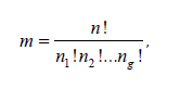
Let j=1, 2, . . . , n index the subjects, where subject j would have a binary response xij under treatment Ti, for i= 1, 2, . . . , g. Assume there are a total of n =n1+n2+· · ·+ng subjects, with ni subjects randomly assigned to treatment group Ti. The number of possible treatment assignments is given by the multinomial coefficient

and each assignment is equally likely with probability 1/m.
The observed outcome for subject j is then represented by the random variable

where Ijk is the random indicator variable that subject j received treatment Tk. To test the null hypothesis, we may use the test statistic

Where  is the treatment level sample proportion, i=1, 2,..,g,
 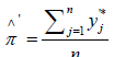 and
and  is the overall sample proportion.
The exact permutation p-value is then computed as:

Where  is the value of the test statistic under the k-th permutation of treatment assignments.
As before, since enumeration of all possible treatment assignments may be computationally prohibitive for large n, we employ a Monte Carlo approximation. By randomly selecting B treatment assignments, the p-value can be estimated as

for the alternative hypothesis H1: π1>π2, with analogous expressions for other alternatives.
In parallel, we also consider a bootstrap-like approach, sampling with replacement from the observed outcomes Y. The Monte Carlo approximation to the p-value in this setting follows the same structure as that of the randomization test.
Similar to the two-group setting, the null hypothesis of equal treatment assignment probabilities across g groups, H0: π1=π2= · · · =πg, can be represented using a 2×g contingency table. This hypothesis may be tested using the exact chi-square test of independence proposed by Freeman and Halton [10], which extends Fisher’s exact test to higher dimensional tables. Importantly, the exact p-value obtained from the Freeman-Halton test is identical to that of the corresponding randomization test [11], mirroring the equivalence observed in the 2×2 case.
The data described in this subsection may also be represented in a K×g contingency table. Under this representation, the hypothesis stated above can be equivalently tested using the Freeman-Halton extension of Fisher’s exact test, which provides an exact chi-square test of independence for multirow by multicolumn tables [12].
In this note we extend these ideas by developing a new approach to resampling based on a Monte Carlo resampling approach. Section 2 introduces our perturbation randomization framework, detailing both the with replacement (WR) and without replacement (WOR) variants and supplying straightforward R code for immediate use. A toy example contrasts the new procedures with Fisher’s exact, Barnard’s, and Boschloo’s tests. Section 3 reports an extensive simulation study that examines the statistical power of each test across a broad spectrum of sample sizes and proportion configurations. Section 4 then analyses two applied data sets, demonstrating how the perturbation tests can alter scientific conclusions relative to traditional exact methods. Finally, Section 5 summarizes practical recommendations.
Perturbation-Based Randomization Testing
The general strategy of our new test involves perturbing the observed data. In the case of Bernoulli outcomes, this means perturbing the binary response (0 or 1). We first describe the method for Bernoulli outcomes in a two-group comparison setting, which naturally generalizes to g-group comparisons for both response types. The perturbations are used to generate a less coarse randomization distribution, while utilizing the original observed test statistic 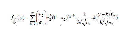 for testing H0: π1=π2 versus the one-sided alternative H1: π1>π2. For the two-sided alternative H1: π1≠π2, we instead use the squared for each subject j, we define the observed outcome as the random variable where Ij=1 if subject j is assigned to treatment T1, and Ij=0 if assigned to treatment T2. Under this setup, x1j and x2j represent the potential outcomes for subject j under treatments T1 and T2, respectively.
To introduce variability for resampling, we generate a perturbed response vector with elements

where the perturbation term ej~N (0, h2), and h is a user specified bandwidth. Unlike traditional smoothing approaches such as kernel density estimation, we fix the bandwidth at h=1/10000, independent of the sample size.
Two resampling strategies are considered: sampling with replacement and sampling without replacement from the perturbed vector Y’. For each resampled dataset, we compute the one-sided test statistic using the estimators

where denotes the resampled value for subject j from the perturbed response vector Y’. For the sampling with replacement approach, we must also use the resampled group mean  when applying the two-sided alternative in two group comparisons, as well as the pooled mean for comparisons involving g groups with binary or multinomial outcomes.
It follows immediately that

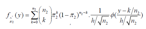
The probability density function (PDF) of 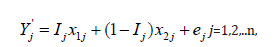 is the following normal mixture:

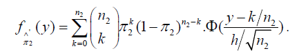
where ϕ is the standard normal PDF. The corresponding cumulative distribution function (CDF) is

where Φ is the standard normal CDF.
Similarly, the PDF of  is
is
and the corresponding CDF is
Thus,  can be interpreted as kernel-smoothed versions of the observed sample proportions
  and
and
 .
.
Each perturbation and resampling iteration yield a value used to construct a Monte Carlo approximation to the null hypothesis distribution. The perturbation-based p-value is calculated in accordance with the exact p-value framework described in Section 1, by comparing the observed test statistic to the distribution of values generated under the null hypothesis. This framework applies equally whether resampling is performed with or without replacement. From the perspective of Monte Carlo inference, this approach offers a practical and conceptually intuitive approximation to the null distribution.
The estimators of the test statistics based on the perturbed responses retain the same expectation as the observed test statistics defined in (1.1) under the null hypothesis H0: π1=π2. The primary motivation for this perturbation-based strategy, particularly in the context of randomized clinical trials, is to achieve Type I error control that more accurately reflects the nominal significance level α. This approach often yields greater statistical power compared to traditional methods such as Fisher’s exact test or the Freeman-Halton extension, especially in scenarios involving small to moderate sample sizes or sparse contingency tables. However, as the sample size increases or the number of treatment arms grows, the advantages of the perturbation-based method tend to diminish, and classical methods generally attain Type I error rates that align with the desired α-level. The extension to the g-group setting follows the same strategy as the two-group case, utilizing the test statistic defined in (1.2).
Toy Examples
To illustrate the differences in p-values obtained using Fisher’s exact test, Barnard’s test, Boschloo’s test, and the proposed perturbation method (under both sampling with and without replacement), we consider a simple toy example for testing the hypothesis H0: π1=π2 versus H1: π1>π2. The observed and perturbed binary data for one Monte Carlo realization, based on a total sample size of n=10, are presented in (Table 1).

The perturbed values y'1 and y'2 corresponding to treatments T1 and T2, respectively, were obtained by adding independent noise to the original binary responses:

where ej~N (0, h) and the bandwidth is fixed at h =1/10000.
Here, Ij=1 if subject j is assigned to treatment T1, and Ij=0 if assigned to treatment T2.
As demonstrated, the resulting perturbed estimators1 and
and closely match their original (unperturbed) counterparts. This confirms that the perturbation does not meaningfully alter point estimation. Both sets of estimators share the same expectation, and the variance introduced by the added noise is negligible.
To estimate the p-value under both sampling with and without replacement, we performed 10,000,000 Monte Carlo resamples. This large number of replicates effectively approximates the full permutation distribution of the test statistic and is computationally efficient in R. Below is the R code used to generate the p-values for testing H0: π1=π2 versus H1: π1>π2:
h <- 1/10000
y0 <- c (1, 0, 0, 0, 0, 0, 1, 0, 0, 0)
y1 <- c (0, 1, 0, 1, 0, 1, 1, 0, 0, 1)
# Observed difference in sample proportions
Obs_diff <- mean(y1)-mean(y0)
# Combine groups
combined <- c (y0, y1)
n <- length(y0) # assumes equal group sizes
# Without replacement: perturb and resample
perm_diffs_wor <- replicate (1e7, {fuzzed <- combined+rnorm(length(combined), mean=0, sd=1) *h shuffled <- sample(fuzzed) mean(shuffled[(n+1) :(2 *n)])-mean (shuffled [1: n])})
pvalue_wor <- mean (perm_diffs_wor >=obs_diff)
# With replacement: perturb and resample with replacement
perm_diffs_wr <- replicate (1e7, {fuzzed <- combined+rnorm(length(combined), mean=0, sd=1) *h shuffled <- sample (fuzzed, replace=TRUE) mean(shuffled[(n+1) :(2 *n)])-mean (shuffled [1: n])})
pvalue_wr <- mean (perm_diffs_wr >=obs_diff)
To compare the behavior of different exact and approximate methods for testing H0: π1=π2 versus H1: π1>π2, we computed p-values using Barnard’s test, Boschloo’s test, Fisher’s exact test, and our proposed perturbation method under both with-replacement (WR) and without-replacement (WOR) resampling schemes. The observed p-values are summarized below: (Table 2.1)
These results demonstrate that the proposed perturbation approach, particularly with sampling with replacement, can yield p-values aligning more closely with Barnard’s and Boschloo’s methods. Notably, the WR method produced the smallest p-value, suggesting increased sensitivity to detect differences under small-sample conditions. In the following section, we further evaluate the perturbation method through a comprehensive simulation study, examining its power and Type I error performance in the two-group, g-group, and multinomial testing settings.
To evaluate the reproducibility of the estimated p-values across multiple executions of the same program, we ran the procedure ten times using the same data. The results for the two perturbation strategies, without replacement (WOR) and with replacement (WR), are shown in the Table 2. As can be observed, the estimated p-values are highly consistent across all runs. Importantly, no decision regarding the null hypothesis H0: π1=π2 versus the alternative H1: π1>π2 would change under either α=0.05 or α=0.10, both commonly used significance levels in clinical trials (Table 2).


Simulation Study
In this section, we compare the new WOR and WR approaches in three settings: the two-group binary outcome setting and g-group binary outcome setting.
Testing binomial endpoints across two treatment groups
In this simulation study, we evaluated Type I error control and power for testing H0: π1=π2 versus H1: π1>π2 using Barnard’s test, Boschloo’s test, Fisher’s exact test, and the newly proposed WOR and WR tests. Values for π1 ranged from 0.05 to 0.95 in increments of 0.10. For each value of π1, corresponding values of π2 ranged from π1 to 0.95, also in increments of 0.10, for sample sizes n=10, 20, 30 per group. The bandwidth parameter h was set to 1/10000. The desired Type I error was set to α=0.05.
For the WOR and WR perturbation tests, 1,000 Monte Carlo resamples were used per scenario to estimate the p-value, and each scenario was simulated 1,000 times. Results for specific combinations of π1 and π2 are reported in (Tables 3-5). Full power curves for each test are shown in (Figures 1-3).


As evident from the results, the WR perturbation test consistently achieves the highest power across all scenarios, with its relative advantage decreasing as sample size increases. The efficiency gains of the WR perturbation test range from approximately 1% to 10%, depending on the parameter configuration. Notably, Barnard’s test tends to outperform Boschloo’s test at lower values of π1, while Boschloo’s test shows superior performance at higher values of π1
Although the performance gain of the WR perturbation test over Barnard’s and Boschloo’s tests may be modest in some cases, it is consistently superior, and in certain settings, the gain is substantial. This improvement can be especially important in clinical trials, such as cancer immunotherapy studies, where even a small reduction in required sample size can lead to significant cost savings. Moreover, the implementation of the WOR and WR perturbation methods is straightforward, as demonstrated by the R code provided in the previous section.

Testing binomial endpoints across g treatment groups
To evaluate the performance of the proposed methods, we conducted a simulation study using 1,000 Monte Carlo replications per scenario and 1,000 resamples to estimate p-values via both the WR and WOR perturbation tests and an approximation to the Pearson exact chi-square test. Type I error and power was assessed under the global null hypothesis for g=3 groups, H0: π1=π2=π3 versus H1: not all πi are equal.
Power was evaluated under various alternatives involving increasing divergence in category probabilities. Across all sample sizes (n=10, 20, 30), both the WOR and WR perturbation tests maintained appropriate control of the Type I error near the nominal level of α=0.05, as shown in (Tables 6-8). The WR method tended to be slightly conservative for n=10. In contrast, the Pearson exact chi-squared test exhibited highly conservative behavior at this smallest sample size, with rejection rates under the null as low as 0.002, although performance improved as sample size increased.


In terms of power, both the WOR and WR perturbation tests consistently outperformed the Pearson exact chi-squared test, particularly at small to moderate sample sizes and under moderate deviations from the null hypothesis. For example, when π1=π2=0.1 and π3=0.5, the WR method achieved powers of 0.580, 0.877, and 0.979 for n=10, 20, 30, respectively, compared to 0.456, 0.844, and 0.970 for the Pearson exact chi-squared test (see corresponding rows in Tables 6-8). Similar patterns were observed in other configurations. When the effect size was large (e.g., π1=π2=0.1, π3=0.9), all three methods approached maximum power even at the smallest sample size.
Overall, these results demonstrate that the WOR and WR perturbation tests offer superior performance in terms of both Type I error control and statistical power, especially in small-sample settings where the assumptions of the chi-squared test may be violated. Among the two resampling-based methods, the WR perturbation test provided the best overall performance, consistently balancing Type I error control and power across all scenarios.
Design Examples
To guide study planning for the one-sided hypothesis H0:π1=π2 versus H1: π1>π2, we first computed the per group sample size n required by Boschloo’s test to attain 80% power at the α=0.05 level. The resulting n values for several (π1, π2) configurations are listed in (Table 9).

Three findings stand out.
•
Fisher’s exact test is markedly under powered relative to the other four procedures.
•
Contrary to common belief, Boschloo’s test does not always dominate Barnard’s test; in some settings Barnard offers comparable or even higher power.
•
The WR perturbation test uniformly outperforms all competitors.
Because real-world conclusions frequently hinge on p-values that lie near the significance threshold, the choice of test can materially affect inference; this will become evident in the applied examples of the next section. Finally, we assessed computational burden for the setting π1=0.35, π2=0.55 with n=75-85. Power curves for the WOR and WR perturbation methods were produced in minutes on a standard desktop, whereas Boschloo’s evaluations stalled for several days without finishing, underscoring its limited practicality for large sample analyses.
Data Examples
Testing Binomial Endpoints Across Two Treatment Groups
The following example, which compares several statistical methods for testing binomial endpoints between two treatment groups, is adapted from the study by Ajani et al. [13]. In this trial, trimodality eligible patients were randomized to receive either no induction chemotherapy (IC; Arm A) or IC consisting of oxaliplatin and fluorouracil (Arm B), followed by concurrent chemoradiation with oxaliplatin/fluorouracil and radiation therapy. One of the primary endpoints was the pathological complete response (pathCR) rate. A total of 55 patients in Arm A and 54 patients in Arm B underwent surgery.
We utilized 100,000 resamples to calculate the WR and WOR perturbation test p-values for testing the null hypothesis H0: π1=π2 versus the alternative H1: π1≠π2. The observed pathCR rates were 13% (7 of 55) in Arm A and 26% (14 of 54) in Arm B. Results from several statistical tests are summarized below:
•
Fisher’s exact test (two-sided): p=0.094
•
Barnard’s test: p=0.082
•
Boschloo’s test: p=0.084
•
WOR test: p=0.073
•
WR test: p=0.081
The primary hypothesis was evaluated at a significance level of α=0.05. As shown, none of the tests reached conventional statistical significance, although the WOR and WR perturbation tests yielded relatively smaller p-values compared to traditional exact tests.
If, hypothetically, the observed pathCR rates were instead 13% (6 of 54) in Arm A and 26% (14 of 54) in Arm B, the test results would be:
•
Fisher’s exact test (two-sided): p=0.081
•
Barnard’s test: p=0.065
•
Boschloo’s test: p=0.058
•
WOR test: p=0.053
•
WR test: p=0.048
In this scenario, the WR perturbation test demonstrated in our simulation study to maintain appropriate Type I error control while offering consistently greater power, would lead to a different conclusion, suggesting statistical significance, unlike the more conservative traditional tests.
Testing Binomial Endpoints Across g Treatment Groups
For this example, comparing Pearson’s exact chi-square test with the WR and WOR perturbation tests, we utilized data from a multicenter, randomized controlled trial conducted across 20 Japanese medical institutions [14]. The study compared three biologics, namely, Infliximab (IFX), Vedolizumab (VED), and Ustekinumab (UST) as treatment arms. The primary endpoint was the clinical remission (CR) rate at week 12, with secondary endpoints including the treatment continuation rate at week 26 and adverse events (AEs). The observed CR rates at week 12 were: 36% (12 of 33) for IFX, 32% (11 of 34) for VED, and 43% (13 of 30) for UST. We used 100,000 resamples to approximate p-values for the exact Pearson chi-square test, the WR perturbation test, and the WOR perturbation test when testing the null hypothesis: H0: π1=π2=π3 versus H1: not all πi are equal.
•
Pearson exact chi-square test: p=0.675
•
WOR test: p=0.663
•
WR test: p=0.649
For the secondary endpoint of rectal bleeding score of 0 at week 1, the rates were: 39% (13 of 33) for IFX, 50% (17 of 34) for VED, and 70% (21 of 30) for UST. The corresponding p-values were:
•
Pearson exact chi-square test: p=0.052
•
WOR test: p=0.043
•
WR test: p=0.044
In this case, different conclusions would be drawn from the WR and WOR tests as compared to the Pearson exact chi-square test at a significance level of α=0.05.
Conclusion
In this note we introduced two new perturbation tests for the hypothesis H0: π1=π2 versus H1: π1>π2 (or π1<π2),
together with the two-sided alternative H1: π1≠π2. The with-replacement (WR) and without-replacement (WOR) perturbation tests are both simple to implement, only a handful of Monte-Carlo resampling lines in R suffice, yet their operating characteristics differ in a way that is practically important. Overall, the WR perturbation test was superior.
Some Key Features of the WR Test
• Consistently higher power: Across an extensive grid of sample size configurations, we benchmarked WR against Fisher’s exact, Barnard’s, and Boschloo’s tests. In every scenario the WR perturbation test delivered the greatest power, with the advantage most pronounced in the small sample setting that dominates Phase I/II clinical trials and rare-event studies. Even a seemingly modest uptick, for example improving power from 0.80 to 0.85, can flip a borderline p-value across the prespecified α threshold, changing the scientific conclusion.
• Exact type-I error control: Like Fisher’s and Boschloo’s procedures, WR maintains the nominal level without the conservatism that plagues Fisher’s exact test. Type-I error protection is therefore not sacrificed for power.
• Generalizes seamlessly: We extended the method to the g-group hypothesis H0: π1=π2= · · · =πg versus H1: not all πi are equal, and demonstrated that WR outperforms the Freeman-Halton exact test while maintaining the desired Type I error rate. The same resampling blueprint naturally accommodates multinomial outcomes, a direction of future work.
• Computational simplicity and transparency: Because the test statistic is distribution-free under H0, Monte-Carlo p-values are obtained in seconds on a lap top, obviating large enumeration tables or specialized software. This lowers the barrier to adoption for practicing analysts.
Conclusion
When a more powerful test requires no additional modelling assumptions, is trivially programmed, and retains exact size, there is little rationale for defaulting to less efficient competitors. The evidence presented here positions the WR perturbation test as the new small sample gold standard for binary proportion comparisons.
Funding
This work was supported by the following NCI grants to Hutson: NRG Oncology Statistical and Data Management Center grant (grant no. U10CA180822); Acquired Resistance to Therapy network (ARTNet) grant (grant no. U24CA274159).
Data Availability
The data used in this study is contained within the manuscript in Section 4.
References
- Rosenbaum PR (2002) Covariance Adjustment in Randomized Experiments and Observational Studies. Statistical Science 17: 286-327.
- Fisher RA (1934, 1970) Statistical Methods for Medical Researchers. Edinburgh, Oliver and Boyd.
- Davis LJ (1986) Exact Tests for 2×2 Contingency Tables. The American Statistician 40: 139-141.
- Barnard G (1945) A new Test for 2×2 Tables. Nature 177.
- Boschloo RD (1970) Raised conditional level of significance for the 2×2-table when testing the equality of two probabilities. Statistica neerlandica 24: 1-35.
- Korn EL, Freidlin B (2024) Design of randomized clinical trials with a binary endpoint: Conditional versus unconditional analyses of a two-by-two table. Statistics in Medicine 43: 3109-3123.
- Mehrotra DV, Chan IS, Berger RL (2003) A cautionary note on exact unconditional inference for a difference between two independent binomial proportions. Biometrics 59: 441-450.
- Lin CY, Yang MC (2008) Improved p-Value Tests for Comparing Two Independent Binomial Proportions. Communications in Statistics-Simulation and Computation 38: 78-91.
- Andr´es AM, Mato AS (1994) Choosing the optimal unconditioned test for comparing two independent proportions. Computational Statistics & Data Analysis 17: 555-574.
- Freeman GH, Halton JH (1951) Note on an Exact Treatment of Contingency, Goodness of Fit and Other Problems of Significance. Biometrika 38: 141-149.
- Agresti A, Wackerly D, Boyett JM (1979) Exact Conditional Test for Cross Classifications: Approximation of Attained Significance Levels. Psychometrika 44: 75-83.
- Mehta CR, Patel NR (1983) A network algorithm for performing Fisher’s. exact test in rxc contingency tables. Journal of the American Statistical Association 78: 427-434.
- Ajani JA, Xiao L, Roth JA, Hofstetter WL, Walsh G, et al. (2013) A phase II randomized trial of induction chemotherapy versus no induction chemotherapy followed by preoperative chemoradiation in patients with esophageal cancer. Annals of Oncology 24: 2844-2849.
- Naganuma M, Shiga H, Shimoda M, Matsuura M, Takenaka K, et al. (2025) Firstline biologics as a treatment for ulcerative colitis: a multicenter randomized control study. Journal of Gastroenterology 60: 430-441.


