Martino Recchia

doi:10.19080/BBOAJ.2024.11.555820

Research Article

Evaluation of the Utility of Pilot Studies in Establishing Bioequivalence

Martino Recchia*

Medistat, Clinical Epidemiology and Biostatistic Unit, Milano; Mario Negri Institute Alumni Association (MNIAA) ,Italy.

Submission: January 18, 2024;Published: March 21, 2024

*Corresponding author: Martino Recchia, Medistat, Clinical Epidemiology and Biostatistic Unit, Milano; Mario Negri Institute Alumni Association (MNIAA) ,Italy, Email id: statmed@hotmail.com

How to cite this article: Martino R. Evaluation of the Utility of Pilot Studies in Establishing Bioequivalence. Biostat Biom Open Access J. 2024; 11(4): 555820. DOI: 10.19080/BBOAJ.2024.11.555820

Abstract

This study aims to assess the actual utility of the sample size tables calculated by Diletti et al. [1] for planning bioequivalence studies. This objective emerged from numerous simulation experiments using data from a real experiment that, during routine statistical analysis (crossover ANOVA), demonstrated complete bioequivalence between reference and test substances.

For each simulated pilot number (N=6, N=8, ..., N=18), we calculated 10,000 %CV values needed to verify the recommended sample size in a real experiment to achieve a bioequivalence response. The comparison between the size proposed by Diletti and that suggested by the simulation was negative due to the high and low under- and over-estimations obtained. Equal estimates were very rare.

We propose conducting a pilot experiment comparing three volunteers in each group. These real data can then be used to simulate 10,000 experiments of 4 vs. 4 and calculate 10,000 Schuirmann tests, checking how often bioequivalence is achieved. If power is below 70%, the next step involves 10,000 simulations of 5 vs. 5, and so on until the desired power is reached. This provides the required sample size [2] for the final experiment.

Keywords: Bioequivalence; Crossover; Sample Size; Resampling; Bootstrap Method

Introduction

To establish a coherent experimental plan for investigating bioequivalence, the following steps are necessary:

i. Determine the required power (70%, 80%, ..., as the probability of correctly establishing the existence of bioequivalence).

ii. Establish an alpha value (5%, 2.5%, ..., as the probability of observing bio-inequivalence).

iii. Calculate a test/reference ratio (Ut/Ur) (0.95, 1, 1.05,...) and a suitable bioequivalence interval (80-125%, ...).

iv. Calculate the sample size for the experiment.

The complex problem raised in step 4 can be addressed by following this strategy:

i. Assume the s2 variability of the parameter (AUC, Cmax).

ii. Select an appropriate experimental design for observations to compensate for potential detrimental effects of variability on the outcome (ANOVA Crossover design - AC).

Unfortunately, the most challenging step is determining the value of s². It is common practice to rely on the results of previous studies or conduct a “pilot trial”.The latter should allow solving the following formula for the sample size suggested by Diletti et al. [1] for the correct size of a trial:

Digression

In a comparative clinical trial, the clinical researcher tries to detect a difference between treatments by ensuring that the study is adequately sized, based on the premise that more observations provide more information. Consequently, the null hypothesis of drugs with the same effect (Ho) will have a high probability of being rejected in favor of the alternative, that the drugs have different efficacy (H1). Experimental pharmacokinetics, however, follows a different path. Here, the scientist tries to validate the null hypothesis Ho to demonstrate that a treatment has at least the same activity as an existing one (bioequivalence). In the domain of statistical inference, however, there is no real reason for such a conclusion. At most, a negative inference test can indicate that the observations made were not actually inconsistent with the null hypothesis Ho. This explains the need to resort to statistical procedures to determine the most appropriate sample size and assess the bioequivalence of the tested drugs (Schuirmann test) [3]. End of digression.

Foot Notes

¹The bootstrap method says: “Define a hypothetical universe - the sample itself - representing the best fit for the real universe. Extract a large number of samples from it and examine the distribution.” The regular method says: “Describe the hypothetical distribution – the normal one - that would have generated the sample. Then use parameters such as the average and standard deviation to describe the distribution. Finally, resort to formulas and tables to verify the features of the samples extracted from that hypothetical universe.”

Methods

s²

Considering the importance of s2, we posed the following question: “Can the coefficient of variation (CV) calculated from s2 obtained in a pilot study indicate the optimal sample size to demonstrate bioequivalence?” To answer this, we analyzed Cmax data from a clinical study on 18 volunteers, following the scheme illustrated in (Tables 1&2).

F treatments=0.02206, F carry-over=0.2069, F period=0.66536 Schuirmann test: t₁=2.4, t₂=4.0, both significant at p<0.01 with 16 df from the AC design. At the conclusion of the statistical analysis, bioequivalence proved indisputable, allowing to virtually consider Cmax as if it came from a single population where we could randomly construct many simulated versions of the experiment presented in Table 2, using a different number of individuals in each replication (our pilot experiments).

Where R= Reference; T= Test

Where Vol.= Volunteers

Simulations – Bootstrap Approach

Search for the smallest number needed to establish bioequivalence

Bootstrap methods are intensive statistical analysis methods that use simulation to calculate standard errors, confidence intervals, and significance tests. The key idea is to sample from the original data, directly or using a fitted model, to obtain replicated datasets from which the variability of the quantities of interest can be assessed without lengthy and error-prone analytical calculations.

From the population in Table 2, we extracted 10,000 random samples [2] of N=18 each. We then calculated the Schuirmann test [3] for each and found that in 75% of the simulations, bioequivalence could be demonstrated with 18 volunteers (75% power). With 16 volunteers, the power was lower, at 71% (Table 3).

Further simulations and Bootstrap samples¹ for the AC design

From Table 2, we selected a first random sample with replacement2 consisting of three volunteers from the RT group (total of six measurements: three in the first period with treatment R and three in the second with treatment T); the second sample included three volunteers from the TR group, following the same criteria as the first (Table 4).

From this information, using the AC design, I obtained the following results for

F treatment = 0.64967 ; s² = 0.06065 ; %CV = 24.9

So I asked: “To what sample size does an estimated %CV from six randomly selected volunteers (Table 4) lead?”

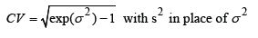
The tables of Diletti et al. [1] provide a number of 20 patients for a power of 70%, α= 5%, Ut/Ur = 1, and a confidence interval for bioequivalence ranging from 0.8 to 1.25. We performed another 9,999 simulations for experiments with three or eight volunteers per group, meaning 9,999 Latin square ANOVAs, as suggested by Jones & Kenward (4). This large number of repetitions ensures considerable stability of the results, allowing a correct interpretation of %CV distributions (one for each N) needed to obtain the proposed 10,000 sample sizes to verify the reliability of power tables. In this case, s² refers to the W-S residual or error (b) of a Split-Plot design; the two values are identical. Diletti et al. [1] argue that to calculate CV, "the mean square of the error, obtained from ANOVA, must be used after transforming the experimental data into LN values."

Foot Notes

²In sampling a finite population, the use of the “with replacement” technique makes the “n” observations independent and equally distributed, validating the Central Limit theorem.

All these simulations led to the following conclusions.

70% Power

The results of the pilot study of 10,000 (Table 5) do not confirm the number of the two Cmax populations we started with (18 volunteers) or the 8 vs. 8, with 16 volunteers, which gave a power of 70%.

The main information obtained from the above table is:

i. the high probability of underestimating the size of the original population

(71.25%, i.e., 1456+...+328=7125/10,000)

ii. the probability of overestimation (19.12%, i.e., 1912/10,000)

iii. the disappointing proportion of “pilot studies” suggesting the correct sizes for the experiment (9.63%, between 16 and 20 volunteers, i.e., 963/10,000).

(Table 6) lists various tables obtained from similar calculations as those discussed but for pilot studies with 8-16 volunteers.

These additional simulations confirm the disappointing sizing information already observed in the study with six volunteers (Table 7).

In conclusion, with every change in N, the probability of underestimating sample sizes increases, the probability of an equal estimate worsens and the probability of overestimation decreases. In any case, this procedure provides disappointing information. Our population consisted of 18 volunteers, and the simulation provided this data with a very low frequency.

The simulation results make the sample size formula shown at the beginning less useful since both the %CV calculation and, subsequently, the sample size calculation is based on hypotheses hardly satisfied in the actual pharmacological response.

80% Power

We repeated the entire procedure, changing the power from 70% to 80%, to operate under more typical conditions of experimental planning. The results of these simulations are represented in (Tables 8,9&10).

Discussion

The width of the simulated confidence interval renders the power sizing tables practically unusable (Table 11). The distribution of residual error obtained from ANOVA applied to data transformed into LN is not what should result from Owen’s algorithm, which is what Diletti et al. used, with some modifications to com-pile their sample sizing tables [2]. Also, t₁ and t₂ use the same error, making it impossible to apply the %CV. However, t₁ and t₂ benefit from the ‘robustness’ of the Student’s t-test, used to calculate them..

Suggestion

A real pilot experiment with six volunteers (3 vs 3) should be conducted. The results could then be used to simulate an initial set of 10,000 t₁ and t₂ calculated for samples with eight volunteers (4 vs 4) using the simulation method; then a second series could be performed, with ..., until 80% of the 10,000 pairs of t₁ and t₂ show bioequivalence. The number, N, confirming this power can then be used for the final experiment. The simulation works quite well with the Schuirmann test, but the use of %CV leads to contradictory results.

References

- Diletti E, Hauschke D, Steinijans VW (1992) Sample size determination for bioequivalence assessment by means of confidence intervals. Int. J Clin Pharm Ther Toxicol 29: 551-558.
- Resampling Stats, Inc. (2000) 612 N. Jackson Street. Arlington, Virginia 22201, USA.
- Schuirmann DJ (1987) A comparison of the two one-sided tests procedure and power approach for assessing the equivalence of average bioavailability. Journal of Pharmacokinetics and Biopharmaceutics 15: 657-680.
- Jones Kenward (2014) design and analysis of cross-over trials, Chapman and Hall CRC.