


Bayesian Mixed Effects Model with Variable Selection
Mingan Yang*
Division of Biostats and Epidemiology, San Diego State University, USA
Submission: June 22, 2020; Published: JAugust 21, 2020
*Corresponding author: Mingan Yang, Division of Biostats and Epidemiology, School of Public Health, San Diego State University, USA.
How to cite this article: Mingan Y. Bayesian Mixed Effects Model with Variable Selection. Biostat Biom Open Access J. 2020; 10(2): 555782. DOI: 10.19080/BBOAJ.2020.10.555782
Abstract
Recently, many approaches have been proposed to address the problem of selecting both fixed and random effects in mixed effects models. In this article, we review several approaches by comparing their procedures and performances, discussing their similarities and differences, and explaining their advantages and disadvantages.
Keywords: Variable selection; Random effects; Mixed effects model; Bayesian model selection; Parameter expansion; Stochastic search
Abbreviations: LME: Linear Mixed Effects; MCMC: Markov Chain Monte Carlo; AIC: Akaike Information Criterion; BIC: Bayesian Information Criterion; GIC: Generalized Information Criterion; SSVS: Stochastic Search Variable Selection
Introduction
Linear mixed effects (LME) models [1] are widely used in longitudinal studies to analyze correlated or clustered data. Generally, the random effects are incorporated to account for heterogeneity among the subjects. In analysis of an LME model, a primary objective is to select potential significant fixed effects and random effects of the outcome variables. Practically, one might be able to use a selection approach (e.g., back-ward elimination or forward selection) and apply a standard criterion, such as the Akaike information criterion (AIC), generalized information criterion (GIC), Bayesian information criterion (BIC), and Bayesian factor, to choose a preferred model by fitting all the possible models repeatedly. However, the number of competing models increases exponentially with the number of predictors. Thus, there are many challenging issues associated with the problem of joint selection of both fixed and random effects such as: intense computation, increased prediction error with increased number of covariates [2], bias associated in estimated variance of the fixed effects and near singular random effect covariance matrix for underfitting and overfitting of the random effects, respectively [3]. In this paper, we review several exemplary approaches by comparing their procedures and performances, investigating their similarities and differences, and explaining their advantages and disadvantages.
The Method
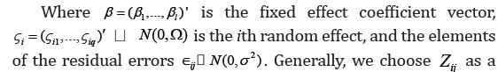
Suppose we have n subjects in a study and each subject has ni repeated observations. For i=1; … , n. Let yij denote the response variable for subject i at observation j; Xij the corresponding l x 1 predictor; and Zij a predictor vector of dimension q x1. Then, we de ne the LME model as follow:

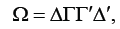
Chen & Dunson [4] addressed the problem by using the reparameterization approach of a modified Cholesky decomposition of the random effects covariance matrix. The covariance Ω can be decomposed as
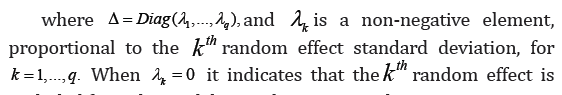
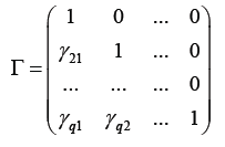
with all diagonal elements being 1 and the other free elements characterizing correlations between the random effects. With this random effects covariance matrix decomposition, model (1) takes the form:

Chen & Dunson [4] showed that by rearranging terms, the covariance matrix of the random effects can be expressed
The priors are specified as follows. Let
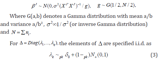
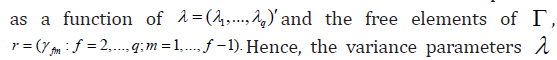
where IG(.) is an inverse Gamma distribution, 0(.)δdenotes a point mass at zero, N+(.) is a truncated positive normal distribution. The lower triangular free elements of Γ is put a normal distribution prior. For easy notation, we denote above zero-inflated truncated positive normal prior as ,~(0,1)kpkZINλ+. g is put a Gamma prior G(1/2; 1/2) and 2σa Jeffrey’s prior 21σ=or an inverse Gamma prior.
Chen & Dunson [4] specified the prior ~(0,).iNIξ Kinney & Dunson [6] used the approach of Gelman [7] and specified the covariance matrix ()(1,...,)iqVDiagddξ−. With this specification, the parameters ,ΔΓand ()iVξare not identifiable. In fact, Kinney & Dunson [6] took the parameter-expansion approach [8,9] that improved computational efficiency and reduces dependence among the parameters. We should note the Chen & Dunson [4] only considered variable selection of random effects. Kinney & Dunson [6] extended it to joint selection of both fixed and random effects for linear and logist models; in addition, the approach of Kinney & Dunson [6] also overcame the computational inefficiency due to slow mixing of the Gibbs sampler
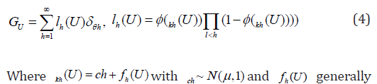
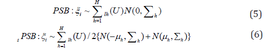
Although it is simple and convenient to assume that the random effects are normally distributed. However, there are several limitations with such specifications: the assumption is often not reasonable; thus misspecification of random effects might result in misleading interpretation and even incorrect results. In addition, it is challenging to specify nonparametric distribution for the random effects since there is bias associated with fixed effects estimates when the expected values of random effects are not zero. To resolve the bias of random effects, Yang [10] and Yang (2013) [11] used the approaches of the Probit stick-breaking (PSB) and location-scale symmetrized PSB (sPSB) [12] for linear and logist models with joint variable selection for both fixed and random effects. They define
Yang (2012) [10] & Yang (2013) [11] provided nonparametric approaches for linear and logist models for joint variable selection of both fixed and random effects. Their approaches are much more flexible than those of Chen & Dunson [4] and Kinney & Dunson [6]. However, the computation is more intense. Later Yang et. al. [13] used the shrinkage priors for mixed effects models with variable selection. The approach is efficient in shrinking small coefficients to zero while minimally shrinking large coefficients due to the heavy tails. They use several popular shrinkage priors: generalized double pareto prior [14], the horse shoe prior [15], and normal-exponential-gamma prior [16], respectively, as follows for the fixed effects:
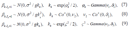
where Ca+(0; c) denotes a standard half-Cauchy distribution on the positive reals with scale parameter c. The performances of the shrinkage approaches are very good while the computations are not that intense.
Conclusion
In this article, we reviewed several approaches of linear and logistic models for joint selections of both xed and random effects. The approaches of Chen & Dunson [4] and Kinney & Dunson [6] are simple in implementation and provide reasonably good results. The approaches of Yang (2012) [10] & Yang (2013) [11] are much more flexible and provide much better results though the computations are intense. The approach of Yang et.al. [13] maintains a good balance of benefits of the above-mentioned parametric and nonparametric approaches. In summary, the performance and computation intensity by descending orders are Yang (2012) [10] & Yang (2013) [11], Yang et al. [13], Chen & Dunson [4] and Kinney & Dunson [6].
References
- Laird N and Ware J (1982) Random-effects models for longitudinal data. Biometrics 38(4): 963-974.
- Miller A (2002) Subset selection in regression. In: 2nd (), Boca Raton, Chapman and Hall/CRC, USA, pp. 1-256.
- Lange N, Laird, NM (1989) The effect of covariance structures on variance estimation in balance growth-curve models with random parameters. Journal of the American Statistical Association 84(405): 241-247.
- Chen Z, Dunson DB (2003) Random effects selection in linear mixed models. Biometrics 59(4): 762-769.
- Zellner A, Siow A (1980) Posterior odds ratios for selected regression hypotheses. Hypothesis Testing 31: 585-603.
- Kinney SK, Dunson DB (2007) Fixed and Random E effects Selection in Linear and Logistic Models. Biometrics 63(3): 690-698.
- Gelman A (2005) Prior distributions for variance parameters in hierarchical models. Bayesian Analysis 1(3): 515-534.
- Liu C, Rubin DB, Wu YN (1998) Parameter expansion to accelerate EM: the PX-EM algorithm. Biometrika 85(4): 755-770.
- Liu JS, Wu YN (1999) Parameter expansion for data augmentation. Journal of the American Statistical Association 94(448): 1264-1274.
- Yang M (2012) Bayesian variable selection for logistic mixed model with nonparametric random effects. Computational Statistics and Data Analysis 56(9): 2663-2674.
- Yang M (2013) Bayesian nonparametric centered random effects models with variable selec-tion. Biometrical Journal 55(2): 217-230.
- Pati D, Dunson DB (2010) Bayesian Nonparametric regression with varying residual density. Annals of the Institute of Statistical Mathematics 66: 1-31.
- Yang M, Wang M, Dong G (2020) Bayesian variable selection for mixed effects model with shrinkage prior. Computational Statistics and Data Analysis, 35: 227-243.
- Armagan A, Dunson DB, Lee J (2013) Generalized double pareto shrinkage. Statistica Sinica 23(2013): 119-143.
- Carvalho C, Polson N, Scott J (2010) The horseshoe estimator for sparse signals. Biometrika 97(2): 465-480.
- Griffin J, Brown P (2007) Bayesian adaptive lassos with non-convex penalization. Australian & New Zealand journal of Statistics 53(4): 423-442.


