Review Article

An Application of Sinc Function based Quadrature Method in Statistical Models

Altaf H Khan*

King Abdullah International Medical Research Center, National Guard Health Affairs, Kingdom of Saudi Arabia

Submission: June 18, 2019; Published: May 22, 2019

*Corresponding author: Altaf H Khan, King Abdullah International Medical Research Center, National Guard Health Affairs, Riyadh, Kingdom of Saudi Arabi

How to cite this article: Altaf H Khan. An Application of Sinc Function based Quadrature Method in Statistical Models. Biostat Biometrics Open Acc J. 2019; 9(4): 555768. DOI: 10.19080/BBOAJ.2019.09.555768

Abstract

The overall goal of this work is to make numerical comparison of Sinc function based method versus other quadrature rules utilized in statistical modeling. Some typical test examples were used to demonstrate the applicability of Sinc quadrature. Results had shown that the it has great potential to be utilized in statistical modeling, since the order of convergence is exponential, works very well in the neighborhood of singularities, in general quite stable and provide high accurate with double precisions estimates.

Abbrevations: SAS: Statistical Analysis Software; GLM: Generalized Linear Model; GLMM: Generalized Linear Mixed Models; ML: Maximum Likelihood; MLE’s: Maximum Likelihood Estimates; EM: Expectation- Maximization Algorithm; FFT: Fast Fourier Transform

Introduction

With the fast pacing and rapidly changing environment from the advent of Pascal’s simple calculating machine to today’s high performance computers now it’s possible to solve complex and intricate problems by utilizing numerous efficient numerical methods, as these numerical methods are the only ultimate choice to rely on since analytical or closed form solutions are either unavailable or could not be obtained. Henceforth, these scientific computational methods are desiderata of any mathematical models whether its formulation is based on deterministic or probabilistic approaches. Whereas, the statistical models are totally based on probabilistic ideas and are commonly observational or experimental data. Moreover, as this era is the century of the ‘Information’, whereas the source of information is in the form of the ‘Data’. While the today’s data is mammoth, huge and gigantic in nature and emerging from diverse field of studies such as from astronomy to the medical imaging. For example, according to in a special report published by ‘The Economist’ data is everywhere: the Sloan Digital Sky in New Mexico (USA) collected the data in few weeks were almost equivalent to what it had collated in the whole history of astronomy, and within a decade it’s archive had 140 tetra-byte of information, whereas radiological modalities are generating thousands of images in few seconds [1-12]. Henceforth, it requires an amalgam of computational scientists to unify the computational tools and techniques at a converging platform where an astrophysicist and a radiologist may have a better discourse on some common issues and could play a pivotal role to uncover the some of mystery of the nature’s complex phenomenon.

A summary of this paper is as below:

First, it gives a general outlines of the Generalized Linear Models, as well as the it’s extended models such as Generalized Linear Mixed Models. Next section deals with some definitions and mathematical theorems related with Sinc function and adopted from Dr. Stenger’s book [1] and also briey explains the Gaussian quadrature rules, as they are most commonly been used in statistical software packages such as SAS (Statistical Analysis Software), Stata and R packages. The Results and Discussion section presents few typical examples of the quadrature integrals and will be compared with the Sinc based quadratures, and conclusion with future work will be given. In this paper only some test functions will be shown and discussed, and the detail results dealing with Sinc based quadrature rules to apply in GLMM algorithms is under progress [13-17]. It seems that this is the rst paper which attempted to apply Sinc Based Approach as it has nowhere been utilized in statistical literature, and only an exception to the Sinc based methods in vast statistics field is by Robert Strawderman [16] from Cornell University, published in StatisticaSinica 2004’s paper: Computing Tail Probability

Statistical Models

As the theory of generalized linear model (GLM) had been unifided by McCullagh & Nelder [5] in 1989, as well as Nelder & Wedderburn [4] as the response variable or dependent variable could assume different type of probability distributions such as discrete or continuous. Basically, the GLM 1 has three main components as below:

The random component: The response variable in the GLM could be the family of exponential function or any discrete outcome variables like Poisson, Bernoulli, and Binomial, and selects the probability distribution.

The systematic component: The systematic component deals with the independent variables and of the form as:

and this combination of predictors is simply the known as the linear predictor.

The link function: The link function is establishes a relation

notation is can be described as below:

whereas this function g(.) connects the random and systematic components.

As the fixed effects models assume that all the observations must be linearly independent of each other, and violation of this assumption may lead to the inapplicability of these models. Hence, to analyze correlated data such as repeated measures analysis of variance, longitudinal data analysis, hierarchical or clustered data, so for such studies a random cluster and or subject effects should need to be included in the regression model as to take into account correlation of the data. So, consider i denote the level-2 units whereas j denote the level - 1 units, further assume that there are i=1,2,....,N subjects and j=1,2,...,ni repeated measures within each subject. A simplest mixed model would be a random-intercept model for subject i is given by

where vi is the random effect for each subject, and the expected value of the response variable is related to the predictor through the link function as:

Now, extending the above model by including multiple random effects and the model would be given as:

where vi is a vector of random effects and should have multivariate normal distribution with mean vector 0 and variance-covariance matrix ;vΣ and the conditional mean ijμ is ,.ijiijEYvx Furthermore, based upon the response variable such as: dichotomous, ordinal, nominal, counts (Poisson), the generalized linear mixed models (GLMM) could be modeled via the link function g(.), detail description could be found in Nicole Michel [14] as well as Jiming Jiang [15] and some other textbooks. The estimation of the parameters is usually done by the maximum likelihood (ML), along with heavy use of numerical computation. As it is clear that the nature of the probability distribution dictates the form of the response variable. Consider ()ijiPYv be the conditional probability for any kind of response distribution and Yi conditional on vi is equal to the product of the probabilities of the level-1 responses as below:

And the above represents the conditional independence assumption, i.e., a subject’s responses are independent give the random effects., and the marginal density of Yi could be given as the integral of the conditional likelihood l(.)

where f(vi) is the distribution of the random effects, assumed to be having multivariate normal distribution. Furthermore, similar integral as above also appears in Bayesian inferences, and is based upon the following steps as:

a) Specifying an unknown parameter values in a probability model which requires some prior knowledge about the parameters,

b) Updating knowledge about the unknown parameters by conditioning this probability model on observed data, and

c) The fit model of the model need to be evaluated for the data and the sensitivity of the conclusions to the assumptions.

According to the Bayes’ law:

where R is the observed data. Moreover, the integral as above appears to be ubiquitous in other scientific computation field such as in modeling credit risk, stock exchange, learning machine, etc., where as in deterministic models, namely as in the numerical computation of parabolic, elliptic, and hyperbolic type partial differential equations where closed form integral are intractable, and only approximation based approach is only available. The maximum likelihood estimates (MLE’s) are done in general via the approximate methods such as:

a. Penalized Quasi Likelihood,

b. Laplace Approximation,

c. Gauss Quadratures, and

d. Markov Chain Monte Carlo.

Penalized Quasi Likelihood and Laplace Approximation’s related work could be found in Tierney & Kadane [8], Breslow & Clayton [7], and Breslow & Lin [6]. Whereas, utilizing Markov Chain Monte Carlo has been also utilized to compute the above integral, a discussion could be found in the work of Sun & Ronnegard [9], also EM (Expectation- Maximization Algorithm) would be utilized but it’s slow. Adaptive Quadrature rules were used in Rabe-Hesketh, et al. [10]. The next section presents an outline for the Sinc function related stuffs [18-20].

Sinc Function based Quadratures Rules

As Cardinal Pope beautifies the sainthood, Professor Frank Stenger had coronated with jewel the cardinal basis function commonly known as Sinc function, as this function is the support when the solution for complex integrand with singularities may not be feasible and could not be achieved by currently available almost all the existing computational techniques, and it is expected that Sinc based approximation will excel for such intricate integrand with achievable precision and accuracy. Now, a brief outline is shown in the following paragraph for Sinc function based approach to compute the integrand. In mathematical literature sinc function as define as:

where Z is dene over the real and complex plane. Moreover, for an arbitrary k and a positive number h, as shown in Dr. Stenger’s book [1] the Sinc function is defined as below(some definitions and theorems are adopted from his book on Sinc Function as well. Dr. Stenger in his book, explained that the sinc function has come from B-spline as follows:

So as N →∞, then the following relation holds

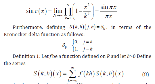
As the series in equation (9) converges, is known as the Whitaker cardinal series for f at h. Next now define the Paley- Wiener class of functions B(h) as follows:

Definition 2: Let h be a positive constant. The Paley-Wiener class of function B(h) is the family of entire function f such that f ∈L2 (R),and in the complex plane f is of exponential type , h π i.e.,

The following two theorems will be useful for interpolation and quadrature formula in B(h)

Theorem 2 Let fϵB(h) then for all ZϵC

The above results for interpolation and quadrature are exact in nature, whereas for fϵB(h), for quadrature the approximation based techniques would be described on a strip Dd

Definition 3: Consider Dd is an infinite strip domain of domain with width of 2d. For d >0

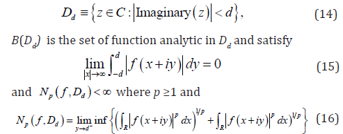
The following result will be give the error bound

Theorem 4 Assume fϵB(Dd) and f satisfy a decay condition of the form

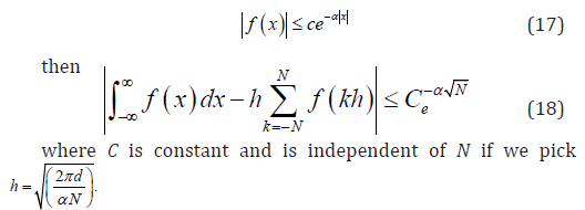
Gaussian Quadratures

As the numerical computation of integrals become necessary when integrand is complicated and become intractable, for example as it’s arise in equation (6) and (7) in the likelihood computation or posterior distribution of the integrals, hence consider the general form as

is single variable. To approximate this integral, consider a finite number of values of the integrand f as:

and define a quadrature as:

whereas wi, for i=0,1,2,...,n are the coefficients known as weights and will be determined for all xi[a,b] where i=0,1,2,...,n are the distinct points in the interval [a,b] (see: Khuri [13]). A quadrature rule is known as closed, if the end points of the interval are used, else it is known as open rule as the end points are excluded when the integral is defined over an infinite interval. Moreover, an error estimation must exhibit that for simple polynomial function it needs to be close to zero. And the order of a quadrature formula is defined as the maximum degree m such that the estimated error is zero for all polynomials of degree less or equal to m, and it is given as: e =α f k (ξ ), where α is a constant and ξ ∈(a,b), whereas k is the order of the derivative, and is associated with the order of the quadrature formula. Furthermore, computation of the quadrature formulas is in general based upon fixed nodes such Newton-Cotes formulas, or Gaussian quadratures where the nodes are not fixed and this makes the order of the Gaussian quadrature formula doubled or less. Now, the quadrature rule could be given as:

The above formula is exact when f is a polynomial. Moreover, computation of the weights and nodes for example is shown in work of Golub & Welsch [11]. The most commonly weight functions are given in the Table 1.

Moreover, the choice of the weights give a family of Gaussian

to note that Sinc based quadrature approximation requires some transformation of the integrands and some of the techniques and some of them are as follows:

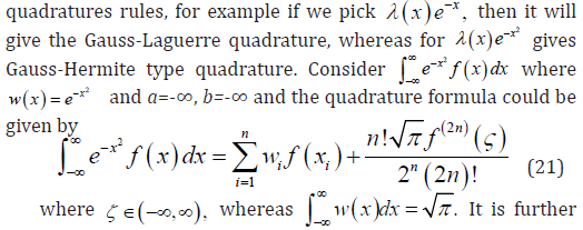
Moreover, the above transformation are only few of them, a complete list of these transformations is provided in Dr. Stenger’s book [1].

Some Results and Discussion

This section discusses some typical test functions and are computed using Sinck Pack and the quadgk. This ‘SincPack’ contains hundreds of routines written in MATLAB (MatheWorks) for solving numerous numerical problems, and it’s available in the ‘Handbook of Sinc Numerical Methods, by Frank Stenger’, at the CRC Publisher’s site:

http://www.crcpress.com/product/isbn/9781439821589.

Whereas ‘quadgk’ could be found in the libraries of MATLAB, this function routine is an adaptive Gauss-Kronord quadrature methods. This quadrature method is expected to be an efficient quadrature rule. And this rule is introduced by a Russian computer scientist Kronord and has better precision than the Gaussian based rules. The computed values for the test functions are shown as below in Table 2 and Table 3. The above results in Table 2 and absolute errors as in Table 3. clearly exhibits that the Sinc quadrature based which is simply based upon the Trapezoidal rule is competing with an adaptive Gauss-Kronord quadrature which is supposed to be highly efficient method and is exact for polynomial of degree 3n+1. Definitely errors shown in Table 3 seems to be better for Gauss-Kronord rule. But surprisingly, this so called most accurate method for the test integral

succumb to fail, as the warning message exactly quoted from the MATLAB is as below:

*****

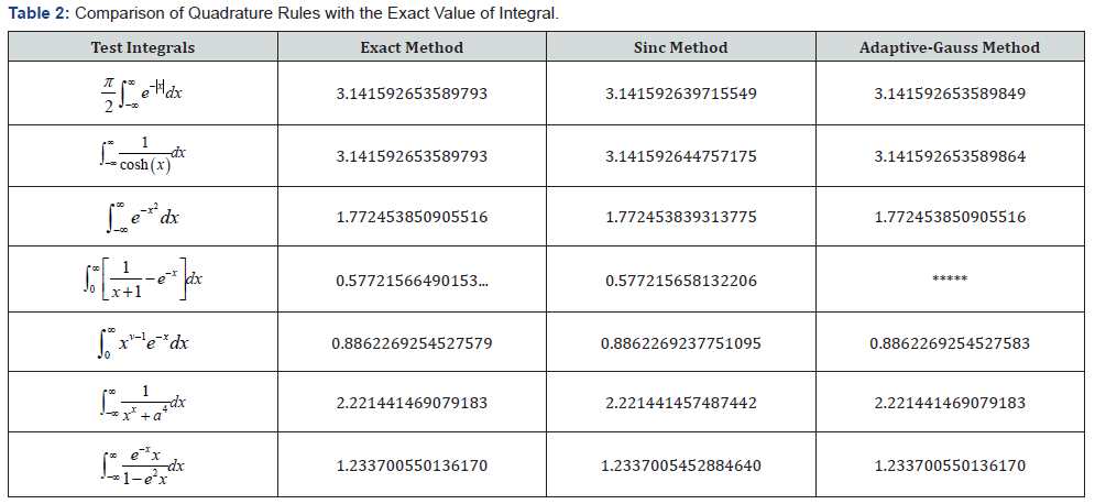
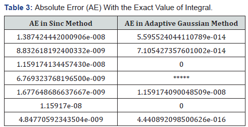
[q,errbnd] = quadgk(@(x) (1./(x+1) - exp(-x)), 0,inf,’RelTol’,1e-8,’AbsTol’,1e-12)

Warning: Reached the limit on the maximum number of intervals in use.

Approximate bound on error is 3.7e+000. The integral may not exist, or it may be difficult to approximate numerically. Increase MaxIntervalCount to 784 to enable QUADGK to continue for another iteration.

> In quadgk>vadapt at 317

In quadgk at 216 q = 5.509872936259971e+001

errbnd = 3.692167159054412e+000

Moreover, as Lawrence F. Shampine [20] had also pointed out similar issue dealing with quadgk, while SincP ack provides a comprehensive approach to deal with intractable integrals. But it should noted be that since the advent of the field of “Numerical Analysis” from Dr. E.T. Whittaker (the first Numerical Analyst) to till today myriad of quadrature rules have been formulated, but the problem is that any of the formula or the algorithm could break down; whereas a comprehensive exposition is available in ‘Numerical Methods and Software’ by David Kahaner, et al. [18]. For

book [18], the estimation of this integral may result an underflow error in the exponential routine, and could be upto -1010 It is almost negligible, whereas setting this underflows as commonly done to set it and set to zero, may cause the estimation of the integral as 0. Furthermore, the standard software such as: SAS, R/Splus, Stata, MATLAB, etc. mostly utilized the adaptive Gaussian quadrature formula have built in function for the generalized linear mixed models. Lessafarre & Spiessens [19] had pointed out that Gauss-Hermite quadrature works well merely for simple problems, but fatally break down for the complicated problems, and they had shown with worked examples MIXOR (by Hedeker and Gibbons), EGRET(Cytel Software Corporation, 1995)), and SAS (SAS Institute, 1999), in general adaptive Gaussian quadrature may work for simple models, but to achieve global maximum is too difficult to get.

Some Future Work Currently we are working on to extend as well as to develop hybrid multidimensional Sinc quadrature rule with most tempting rules would be to utilize the work of Kenneth L Judd and Benjamin S. Skrainka[21], and their work is based on polynomial based rules as well as Clenshaw-Curtis as discussed by Llyod N. Trefethen [3] had shown with examples that Clenshaw-Curtis quadrature method is as good as Gaussian based methods and is easy to implement using Fast Fourier Transform (FFT) as well as with better computational time . A brief outline as below is given for the multidimensional quadrature as below: In general, multidimensional integrals are computed via iterated approach by evaluating a single integral using scalar product rule. Consider an integral in multidimensional as follows:

where Rd is defined over d dimensional space. A product rule to approximate the above integral could be as follow:

Hence, evaluation of a multidimensional integral is done by applying Cartesian or Tensor product rules. Moreover, currently only Monte Carlo based approach is most suitable if it requires to evaluate quadrature integrals in higher dimension, and this approach is last resort for the computational scientists. Some of the attractive features of their paper is:.

i. 10 times more accurate with a given number of nodes,.

ii. it’s faster than almost 10 times,.

iii. Standard errors are accurate, and.

iv. robust and works well for the large datasets, while remarked that pseudo Monte Carlo method is an inaccurate method to compute the integral and results are not reliable..

Moreover, a combination of Smolyak and Sinc quadrature along with Clenshaw-Curtis rule, and these approaches we will explore to utilize in GLMM models for the computation of multidimensional integrals to estimate the random effects.

Conclusion

As the test functions have demonstrated that Sinc based quadrature has shown the computed integrand using Sinc quadrature is comparable to the adaptive Gauss-Kronord rule. It’s algorithm did not break down for any of the test function, hence it shows that it has a viable potential applications and could be craftily used to compute the intractable integrals in Generalized Linear Mixed Models as well as posterior estimation of Bayesian problems. The order of convergence is exponential, and Sinc based methods had already shown a great applicabilities in deterministic problems, and our future work will be based on to exploit it’s nice features for statistical models.

References

1. Frank Stenger (1993) Numerical Methods on Sinc and Analytical Functions, Springer-Verlag, New York, Inc., USA.
2. Legendre, Adrien-Marie (1805) Nouvelles méthodes pour la détermination des orbites des comètes [New Methods for the Determination of the Orbits of Comets] (in French), Paris: F. Didot
3. Llyod N Trefethen (2008) Is Gauss Quadrature Better than Clenshaw-Curtis?, Oxford Computing Laboratory, Wolfson Bldg., Parks Rd., JSTOR 50(1): 67-87.
4. Nelder J, Wedderburn RWM (1972) Generalized linear models. Journal of the Royal Statistical Society A 135: 370-384.
5. McCullagh P, Nelder JA (1989) Generalized Linear Models, (2^nd Edn), Chapman and Hall, London, UK.
6. Breslow NE, Clayton DG (1993) Approximate Inference in Generalized Linear Mixed Models. Journal of the American Statistical Association 88(421): 9-25.
7. Breslow NE, Lin X (1995) Bias Correction in Generalised Linear Mixed Models with a Single Component of Dispersion. Biometrika 82(1): 81-91.
8. Tierney L, Kadane JB (1986) Accurate approximations for posterior moments and marginal densities. Journal of American Statistical Association 81: 82-86.
9. Lei Sun, Ronnegard L (2011) Comparison of Different Estimation Methods for Linear Mixed Models and Generalized Linear Mixed Models, Dalarna University University, Swden.
10. Rabe Hesketh S, Skrodal A, Pickels A (2002) Reliable estimation in Generalized Linear Mixed Models using Adaptive Quadrature. The Stata Journal 2: 1-21.
11. Gene H Golub, John H Welsch (1968) Calculation of Gauss Quadrature Rules. Mathematics of Computation (American Mathematical Society) 23(106): 221-230.
12. (2010) Data; data everywhere 'The Economist', Special report: Managing information.
13. Davis PJ, P Rabinowitz (1975) Methods of Numerical Integration. Academic Press, New York, USA.
14. Khuri AI (2003) Advanced Calculus with Applications in Statistics. John-Wiley & Sons, USA.
15. Nicole Michel (2009) Mixed Effects Models and Extensions in Ecology with R. Springer, Switzerland.
16. Jiming Jiang (2007) Linear and Generalized Linear Mixed Models and Their Applications, Springer, Switzerland.
17. Robert L Strawderman (2004) Computing Tail by Numerical Fourier Inversion: The absolutely Continuous Case. Statistica Sinica 14: 175-201.
18. David Kahaner, Cleve Moler, Stephen Nash (1988) Numerical Methods and Software, Prentice Hall, Englewood Cliffs, New Jersey, USA.
19. Emmanuel Lessafarre, Bart Spiessens (2001) On the effect of the number of quadrature points in a logistic random-effects model: an example. Applied Statistics 50(3): 325-355.
20. Lawrence F Shampine (2010) Weighted Quadrature By Change of Variables Neural, Parallel, and Scientific Computations 18: 195-206.
21. Kenneth L Judd, Benjamin S Skrainka (2010) High performance rule: how numerical integration affects a popular model of product differentiation, cemmap working paper CWP03/11, Centre for Microdata and practice, The Institute of Fiscal Studies, Department of Economics, UCL.