Wave Patterns of Annual Global Carbon Dynamics (According to information Global_Carbon_Budget_2017v1.3.xlsx)
Mazurkin PM*
Professor, Volga State University of Technology, Russia
Submission: July 18, 2018; Published: December 14, 2018
*Corresponding author: Mazurkin PM, Dr. Sc., Prof., Volga State University of Technology, Yoshkar-Ola, Russia
How to cite this article: Mazurkin P. Wave Patterns of Annual Global Carbon Dynamics (According to information Global_Carbon_Budget_2017v1.3.xlsx) . Biostat Biometrics Open Acc J. 2018; 8(5): 555748. DOI: 10.19080/BBOAJ.2018.08.555748
Abstract
The wavelet analysis of the annual dynamics from 1959 to 2016 of six factors of the global carbon budget is carried out by the method of identification and two-term trends and sets of wavelets with variable amplitude and period of oscillations are obtained. The features of changing the parameters of wavelets are shown. Positive and negative wavelets are identified for the growth vector of the global carbon budget. The critical wavelets with amplitude according to the law of exponential growth are shown for the future. In addition to the first term showing the natural process, all other components of the General model characterize, as a rule, natural-anthropogenic or even anthropogenic influence. In this case, the two-term trend is the limit state of two wavelets with a period equal to infinity. More difficult is the study and subsequent change in the effects of ocean and atmospheric emissions. A technological breakthrough in the impact of fossil fuels and industry is needed. The impact of fossil fuels and industry on the carbon budget vector of human behavior is clear – a technological revolution is needed to form a waste-free industry with waste-free fossil fuel technologies. Otherwise, the impact of the ocean on the global carbon budget will only increase.
Keywords: Carbon; Budget; Data; Dynamics; Wavelet analysis; Patterns
Introduction
To model annual global carbon dynamics from data [1] (in the part Historical CO2 budget in the file Global Carbon Budget) we applied wave equations with variable amplitude and period of oscillations. The world has a lot of data by year. It is known [2], for example, that «European forests are intensively exploited for wood products, yet they also form a sink for carbon. … Encouragingly, the environmental conditions in combination with the type of silviculture that has been developed over the past 50 years can efficiently sequester carbon on timescales of decades, while maintaining forests that meet the demand for wood». This and other articles apply linear or reducible equations to linear forms «The aim of Paris Agreement is `holding the increase in global average temperature to well below 2 0C above pre-industrial levels and pursuing efforts to limit the temperature increase to 1.5 0C. The Parties also undertook to achieve this goal by reducing net emissions `to achieve a balance between anthropogenic sources and removals by sinks of greenhouse gases in the second half of this century’, and hence implicitly not by geo-engineering planetary albedo. Under what conditions is this goal geophysically feasible» [3].
We believe that one of the conditions is to identify stable patterns from the accumulated statistical data. And these laws allow you to better understand the past and predict certain possible behaviors of people who make decisions. At the same time, our method of identification of the General wavelet equation (solitary wave) from the measured statistical data will allow to Supplement and clarify the climate mitigation scenarios up to 2100, described in the article [3]. Another condition will be the identification of the scenarios themselves by their quantitative data on the possibility of their reliability. Only those scenarios for which the wave equations of high adequacy will be obtained will be reliable [8-14].
According to the article it is known that “If CO2 continues to rise further into the twenty-third century, then the associated large increase in radiative forcing, and how the Earth system would respond, would likely be without geological precedent in the last half a billion years” [4]. Climate change has been studied here for 420 thousand years. Then all revealed by the past statistical data can be grouped and given on the basis of their analysis plausible scenarios of future behavior of people on our planet. However, even in this article, although the dynamics shows clearly wave changes, only trends are given in the form of linear equations. Our method to identify important primary factors and not their derivatives (estimated). Therefore, the indices proposed in [5] can be used only in assessing the adequacy of the identified wave patterns, but not before their detection. In the article [6], on the basis of the analysis of growth of eight tree species it was revealed that due to global warming in Western Europe there is a slowdown in forest increment. But we noticed that the quadratic equations are applied, the parameters of which do not have physical sense. In our articles on dendrochronology [12,13] and other examples, for example, in the study of a set of genes [14], the same wave patterns are obtained.
The carbon budget depends largely on the scenarios of greenhouse gas changes, which are considered in article [7] up to 2300. In the future, factor analysis of all quantitative scenarios can be carried out to characterize the relationships between individual factors. The method of identification of the generalized wavelet is also used here.
Source data
The Global Carbon Budget 2017 is a collaborative effort of the global carbon cycle science community coordinated by the Global Carbon Project [1]. The symbols of the parameters from the Table 1:
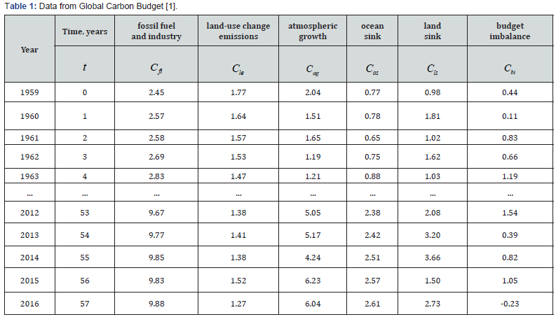
t- Time in years since the initial data were recorded [1], 0t=for 1959;
Cfi- Emissions from fossil fuel combustion and industrial processes (uncertainty of ±5% for a ± 1 sigma confidence level);
Cle- Emissions from land-use change (uncertainty of ±0.7 GtC/yr);
Cag -The atmospheric CO2 growth rate (variable uncertainty around 0.2 GtC/yr from 1980) is estimated directly from atmospheric CO2 concentration measurements, NOAA/ESRL
Cos- The ocean sink (uncertainty of ±0.5 GtC/yr) is estimated from the average of several global ocean biogeochemistry models that reproduce the observed mean ocean sink of the 1990s;
Cls- The land sink (uncertainty of ±0.9 GtC/yr on average) was estimated from the average of several dynamic global vegetation models that reproduce the observed mean total land sink of the 1990s;
Cbi- The budget imbalance is the sum of emissions (fossil fuel and industry + land-use change) minus (atmospheric growth + ocean sink + land sink); it is a measure of our imperfect data and understanding of the contemporary carbon cycle.
Identification method
The modeling concept on statistical selections: Statistical selection – this multiple-factor numerical field issued in the form of tabular model. This definition it significantly differs from tables of statistical researches as only numerical selections are applied to modeling [8-11]. And optional all cages of the table have to be the filled numbers. However, cages have to have quantitative, uniform on the accepted set of factors, values. Thus, the tabular model optional has heuristic explanations. As a rule, authors of measurements, providing in the publications results of researches in the form of tables of data, as a rule, yield incorrect substantial interpretation. Therefore, it is necessary to provide in publications primary data of measurements, instead of transformed by results of application of classical mathematical statistics data.
This phenomenon of formalization is connected with that the table of results of measurements even if it is made by authors correctly, can’t be substantially comprehended without carrying out the factorial analysis (in article it isn’t provided) with mathematical modeling of communications between couples of factors for identification of binary communications. Then primary there is a tabular model (an initial numerical field) which is estimated on an error of measurements, and secondary - the required difficult algebraic equation (in the sense of Descartes), made of invariants (that is Hilbert’s bricks). Primary data invariant in relation to different models. We called this process of identification – statistical identification. The antiderivative in the form of the unknown integrated equation becomes not necessary though, maybe, someone and will manage to receive integrals on our models. It would be great creation, as well as Maxwell’s general equations for electromagnetism.
Determined model: Generally not the wave determined model (for example, a trend or a tendency) contains the sum of two biotechnical laws and receives a type of the equation

Where,
yo– a trend (tendency) of a dependent factor (indicator),
x – an explaining variable,
a1....a8 – parameters of the generalized model (1).
Not the wave nature of the general model (1) gets in two cases:
• when a step of discretization of measurements too big in comparison with the period of oscillatory indignation of measured real process (for example, the impulse of the electrocardiogram demands amplitude registration through everyone 0,001 c);
when the interval of process of measurements is small in comparison with a half-cycle of oscillatory indignation of the measured indicator (for example, change of global average annual temperature in one point of Earth demands registration for 1000 years and more).
Asymmetric wavelet: We adhere to Descartes’s concept about need application of the algebraic equation of a general view directly as final mathematical solution of the unknown differential or integrated equations. For such generalization the new class of wave functions was offered. To conditions of physical existence of the phenomena and processes asymmetric wavelet-function of a look most fully satisfies

Where,
y – an indicator (a dependent factor),
i – number of the making model (2),
m – number of members in model (2),
x – the explaining variable (the influencing factor),
a1....a8 – the parameters accepting numerical values during structural and parametrical identification of model (2).
In most cases for identification of steady biotechnical regularities, because of rather low accuracy of tabular models, the truncated design (on the formula of the period enclosed in trigonometric function or fluctuation frequencies) asymmetric wavelet type is sufficient

The number m of members in our examples up to 120 or more. For example, change of relative atomic mass of chemical elements depending on serial number in D. I. Mendeleev’s table received model with 92 members.
Dynamic range as a series of signals: Physics and Mathematics approach involves understanding dynamic range as a reflection of some composite process or multiple series and parallel occurring natural and/or natural and anthropogenic real processes. For the first time it was succeeded to receive models of many types of series of dynamics on the concept of additive decomposition of any dynamic row on a set of signals.
The signal is a material data carrier. And information is understood by us as an interaction measure. The signal can be generated, but its reception isn’t obligatory. So, for example, a number of prime numbers is known some thousands of years, but its essence as sets of signals still wasn’t opened [5]. Any physical process or its part can be a signal. It turns out that change of a set of unknown signals is known long ago, for example, through ranks of hydrometeorological measurements in many points of a planet. However still there are no statistical models of dynamics of global temperature and other parameters of earth’s environment.
Then we can write down any equation of type (3) as a look wavelet-signal

Where,
Ai – amplitude (half) of a wavelet (axis y),
pi – a half-cycle of fluctuation (axis x).
ip – a half-cycle of fluctuation (axis x). The concept of a wavelet signal allows to abstract from physical sense of statistical ranks of measurements (generally not only dynamic ranks) and to consider their additive decomposition on separate components in a look wavelets. First, the factors were ranked in descending order of the correlation coefficient from the global influence according to the two-term trends of dynamics:
• Fossil fuel and industry 0.9933;
• Ocean’s 0.9820;
• Land-uses 0.8476;
• Atmospheric emission 0.7179;
• Lands 0.4995;
• Carbon budget imbalance 0.3779.
Dynamics of fossil fuels and industry
On the computational capabilities of the software environment CurveExpert-1.40 only the first four components are identified together (Figure 1). A total of 28 members of the General model were obtained (Table 2).
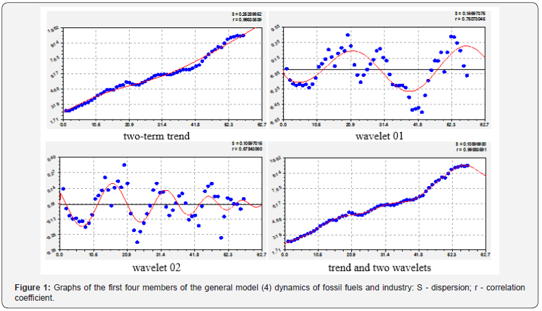
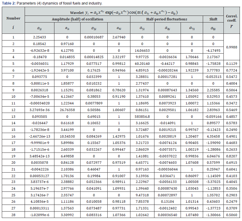
The correlation coefficient of the trend is 0.9933, and with the addition of two wavelets, the adequacy increases to 0.9988. The first term of the trend in table 2 is the law of exponential loss (the Laplace law modified by us) and it characterizes the natural process. According to it, if there was no humanity, there would be a sharp reduction of carbon from fossil fuels and industry. The second term of the trend and subsequent fluctuations, as a rule, show an anthropogenic impact on the dynamics of the indicator. The second term is changed according to the law of exponential growth and has no inhibition yet. In climate mitigation scenarios, first of all, it is necessary to determine the measures for braking, including the amplitude and the law of exponential death, and then the complete exclusion of the second component from the dynamics of this factor.
With the correlation coefficient 0.9843 the dynamics of the factor is shown by the equation of the form

Thus, the main trend is indicative of the law of the anthropogenic influence intensity of growth 1.24184 that much more 1. Table 2 shows that due to the action of the first member of the natural decline, the intensity of the exponential growth is 0.97160, which is slightly less than 1. This means there is little inhibition to further growth of fossil fuel dynamics and industry.
The first and second wavelets in Figure 1 have a negative sign in Table 2, so the fluctuations are a crisis for carbon growth due to the influence of fossil fuel and industry. The first oscillation occurs with a constant half-life of 14.06653 (or a period of about 28 years). Apparently, this growing fluctuation shows the desire of mankind to resist the anthropogenic growth of fossil fuels and industry. Such positive (with a negative sign) for mankind wavelets in Table 2, there are 13. Their amplitude-frequency response will need to pay close attention.
An interesting situation is emerging: according to the latest chart in Figure 1, humanity is trying to resist the growth trend with two crisis wavelets (for the influence of fuel and industry). As a result, it can be seen that the overall schedule of four members from 2017 may decrease and therefore the indicative forecast is to reduce carbon with further increase in fossil fuel production and industry development. Then the only alternative to progress is the transition to waste-free combustion of fossil fuels and the development of waste-free industry technologies.
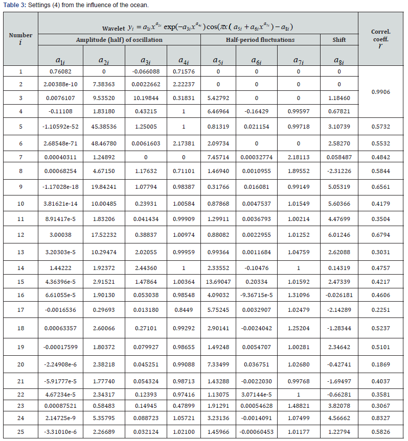
Dynamics of changes from the ocean
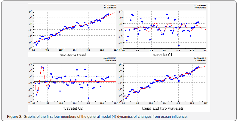
If the previous changes were completely anthropogenic (only people do it), the influence of the ocean belong to the natural processes (Figure 2, Table 3). Unfortunately, the global carbon budget from the influence of the ocean only grows according to the law of exponential growth (the first natural member of the trend). In 1959 and 2016, according to Table 1, the parameter values were equal to: C=fi=2.45 and 9.88; Cos=0.77 and 2.61. Then we get that the increase in the values of the two factors for 57 years occurred, respectively, in 4.03 and 3.38 times. The share of influence of the oceans from fossil fuel and industry equal 31.43 and 26.42%. Thus, the rate and share of carbon growth from the ocean is lower than that of carbon from fossil fuels and industry.
Only one natural component of the influence from the ocean is

If there were no other 24 members of the general model in Table 3, the correlation coefficient (6) is 0.9748. The first four member give value 0.9906. Thus, the introduction of wavelets gives a decrease in the activity of the exponential growth in 0.20677 / 0.066088 ≈ 3.13 times, thus increases the intensity of exponential growth in 0.71576 / 0.46783 ≈ 1.53 times. Accounting for the oscillatory perturbations provides the opportunity to examine any changes in wave dynamics. At the same time we accept the concept of oscillatory adaptation of the Universe, and hence the wave dynamics of natural and anthropogenic processes on Earth. The graphs in Figure 2 show that the second wavelet has long been a history and was completed by 1979. And the first oscillation still continues to operate, apparently, ending by 2040. So, it is possible to perform all the wavelets, leaving to predict only those that continue in time in the future. The fourth member (the second wavelet) received a negative sign and there are 8 of 25 such in Table 3. The seventh term, having the amplitude according to the exponential law, becomes the most dangerous for the influence of the ocean.
Dynamics of changes from land use
Arable land is the most affected by land-use changes. However, the data [1] seems to take into account the average impact of any type of land use. The graphs in Figure 3 show that for the first 20 years from 1959 to 1979, the dynamics of the global carbon budget from the impact of land use decreased. At the same time, there is a gradual change in the factor until 1999. And then there is a transition to a strong oscillatory perturbation with the growth of the influence of land use. This factor moved to tremor. Table 4 shows the model parameters (4) for the 18 members of the general model.
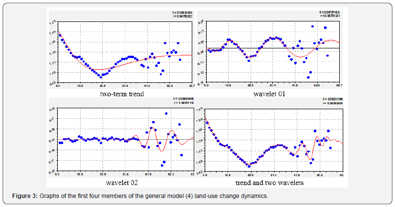
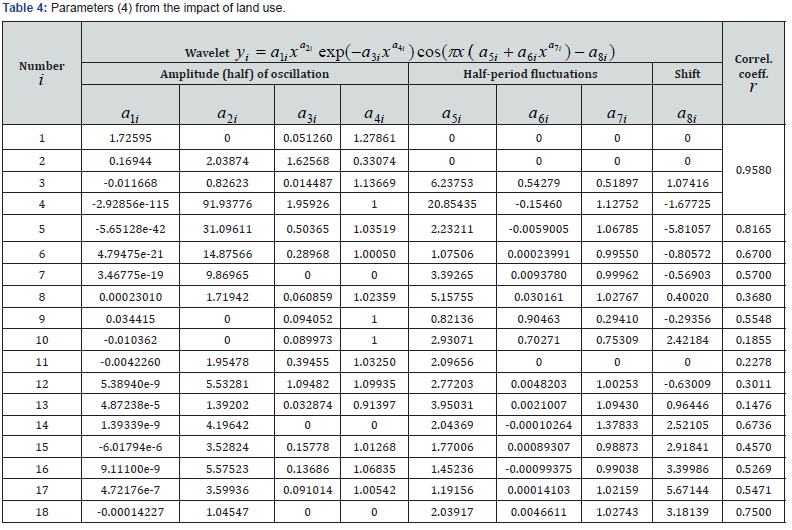
In this regard, the trend contains the sum of the laws of natural exponential death and stress anthropogenic excitation (the so-called biotechnical law of prof. Mazurkin P. M.). Then, as in fossil fuels and industry, the global carbon budget can be managed for this factor. At the same time, we can see from the wavelets in Figure 3 that both of them will be excluded in the future. Therefore, in the future, measures should be taken to exclude the second member, that is, in the global plan to calm the behavior of mankind by measures to mitigate the impact of climate. It will be necessary to manage land use needs, increasing the area of protected areas and forests on the planet. Six wavelets become crisis for the impact of land use (in the direction of carbon reduction). But the wavelets № 7, 14 and 18 become dangerous by the change of amplitude according to the exponential law. Other wavelets have boundaries of change, so they are referred to as finite-dimensional wavelets (really solitary waves, that is, they are solitons).
Dynamics of air emissions
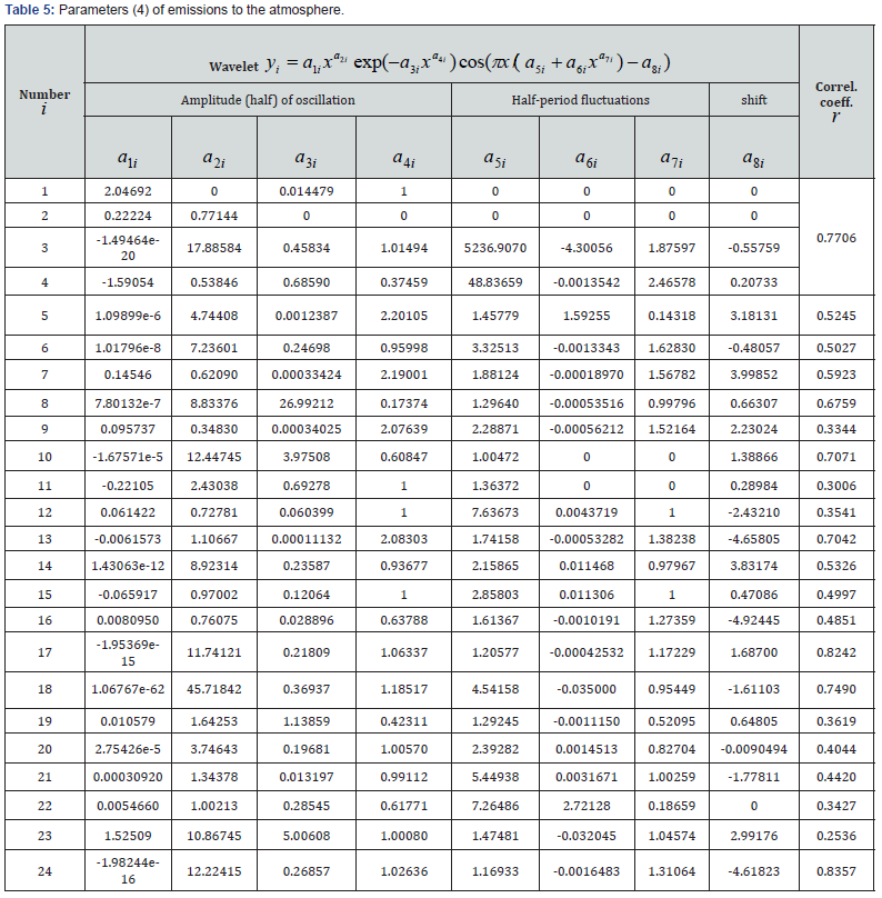
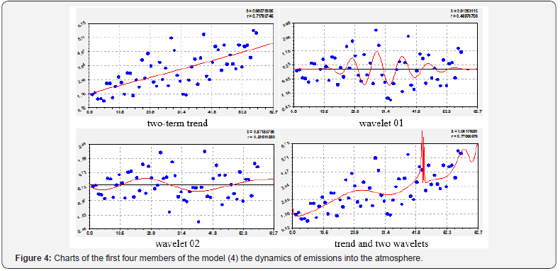
This parameter of the global carbon budget is controversial already in the very laws of the trend (Figure 4, Table 5). The first, and therefore natural, term of the trend under the condition a4i=1 is the Laplace law (in mathematics), Mandelbrot (in physics), pearl (in biology) and Pareto (in the economic metric). However, the trend is almost entirely determined by the second member in the form of the indicative law. Then it turns out that the dynamics of the carbon budget from atmospheric pollution seems to be inverted: the second member of the anthropogenic influence becomes more significant, and the process of natural reduction due to self-purification moves to the distant plan. Two wavelets in Figure 4 due to the negative sign counteract the growth of the influence of air pollution. There are eight wavelets out of 24 such positively directed to purify the atmosphere in Table 5.
Dynamics of changes from the earth’s influence
A similar character is the dynamics of the carbon budget from the influence of the earth on top-news (Figure 5, Table 6). However, in contrast to the influence of the earth, both wavelets have already remained as a historical fact. This was affected by the efforts of environmentalists over the past 50 years. At the same time, the General model received 40 members, of which according to Table 6, 17 members have a negative sign. Then it turns out that the earth (the land of our planet) has the best ability to cleanse. In the simple case, the trend receives a formula with a correlation coefficient of 0.4994 of the form
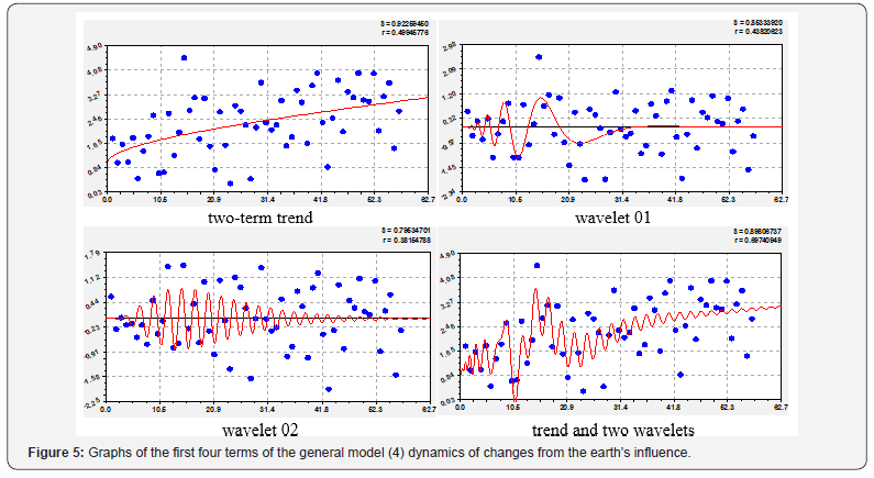
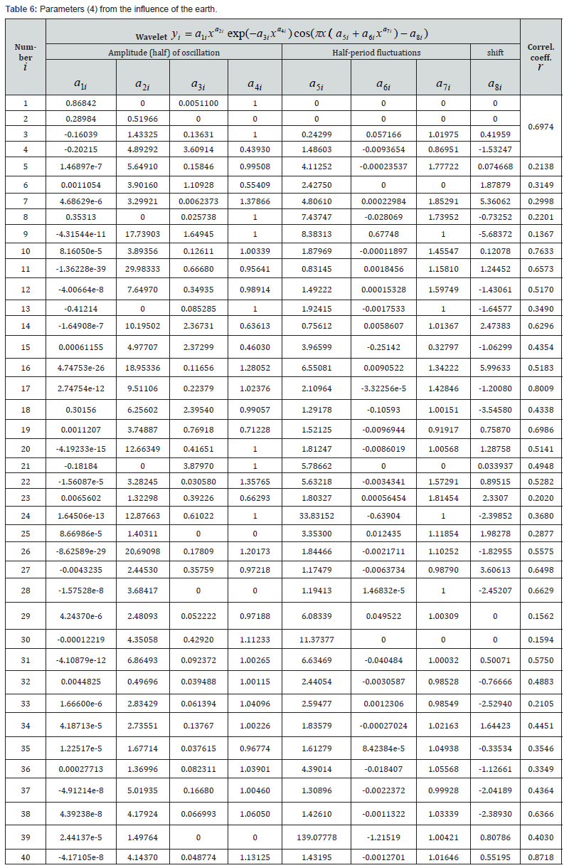

The second term in Table 6 gives the activity of exponential growth by 0.28984 / 0.16830 ≈1.72 times, and the growth intensity by 0.51966 / 0.60771 ≈ 0.86 times less. The ratio of the two-term trend was equal to 0.4995. Thus, even with the adequacy difference of 0.000058, the parameters of the rough (7) and more accurate trends are very different (Table 6). All the wavelets we have received if the correlation coefficient is not less than 0.1. Some wavelets had the adequacy of even more compared to the first four members of: №10 – 0.7633; №17 – 0.8809; №19 – 0.6986; №40 – 0.8718. Thus, each wave shows the degree of its inclusion in the general model relative to the previous residues (absolute error of modeling). This indicates the quality of the original data in Table 1.
Dynamics of the budget imbalance
The budget imbalance factor is more related to statistical indicators of verification of the balance sheet amount by the previous five parameters of the global carbon budget. The two-term trend in Figure 6 and Table 7 shows that the imbalance has increased sharply since the beginning of the 21st century. The first two wavelets are already in history.
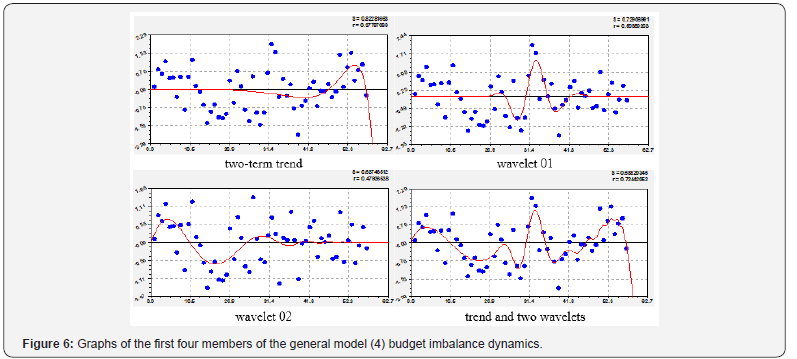
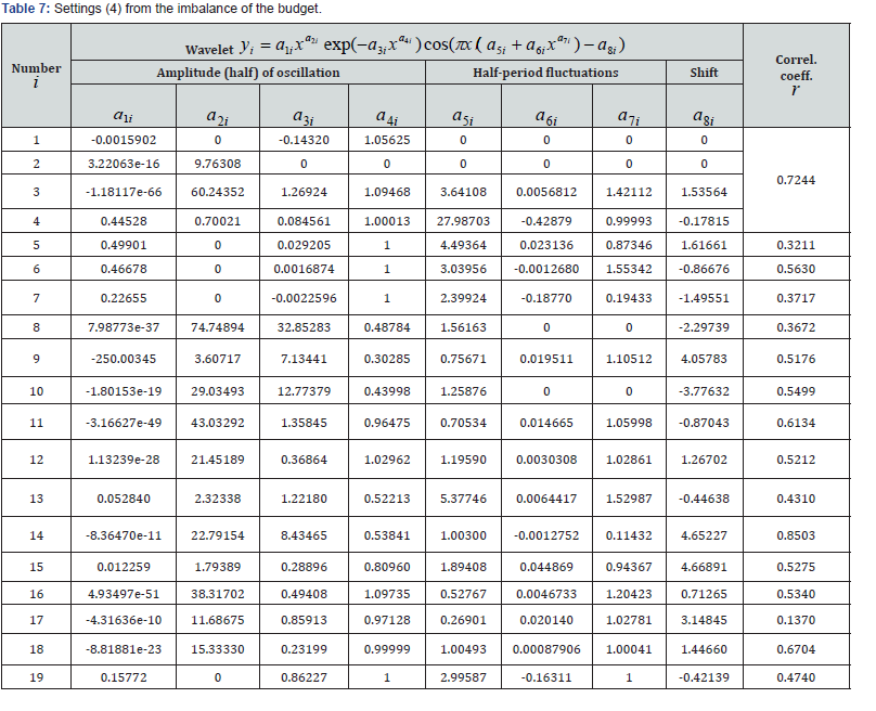
According to the two-term trend, the negative sign before the first member shows the crisis in the budget imbalance, and it increases according to the law of exponential growth. The second member according to the indicative law shows that since 2005 there is a sharp change in the indicator. However, since 2016, the sweat trend is planned again to move to negative values of the carbon budget imbalance.
The adequacy of all detected wavelets allows us to calculate the coefficient of dynamics (Table 8) kof the factor’s influence on the global carbon budget by the formula

Where,
r1+2 correlation coefficient of the two-term trend.
From the graphs in all figures, we obtain for trends a coefficient that takes into account the level of dynamics of processes:
• On the dynamics from 1959 to 2016 of the impact of fossil fuels and industry 1-0.9933 = 0.0067;
• On the dynamics of the influence of the ocean 0.0180;
• On land use change 0.1524;
• On the dynamics of emissions into the atmosphere 0.2821;
• On the dynamics of the impact of the earth’s terrestrial planet 0.5005;
• On the dynamics of the global budget imbalance 0.6221.
Then it turns out that the most changeable were the research processes.
The greater the coefficient of dynamism, the more chaotic the processes. The most dynamic is the imbalance of the carbon budget, but from the standpoint of vibrational adaptation, the worst from the standpoint of management is the dynamics of the impact of fossil fuels and industry. People are gradually increasing the understanding that the growth trend is steadily increasing and there are no solutions to curb this trend. Therefore, the only alternative is a waste-free technological revolution. This will allow to change the structure of formulas of all components of the general model (4) to reduce the impact of all factors.
Conclusion
Using the example of global carbon dynamics from 1959 to 2016, the applicability of the wavelet analysis by the method of identification of the general equation of oscillations with variable amplitude and period of oscillations is proved. The number of detected equations of oscillations depends on the quality of the initial data and measurement error. In all equations of the first four members turned out on the computing power of the software environment CurveExpert-1.40, of which the first two members belong to the trend. We understand the trend as the sum of wave components that have a period of oscillation approaching infinity. Therefore, the trend parameters are recorded in the General table by the oscillation numbers for one factor, and they also belong to the class of wavelets.
There are two types of wavelets:
i. Infinite-dimensional oscillations in which the amplitude varies on the entire axis of the abscissa, and it is identified by the exponential law of growth or death, having no boundaries;
ii. Finite-dimensional wavelets (really solitary waves or solitons) whose amplitude varies according to the biotechnical law in a specific range of abscissa values [10, 11].
As a rule, in geoecological laws infinite-dimensional wavelets show the influence of space objects, including the Earth, and finite-dimensional wavelets often display unconscious or partially conscious behavior of mankind. Therefore, one should simply get used to understanding the oscillatory adaptation of humanity to limited natural resources. To do this, we need to develop wavelet thinking, primarily at all levels of education. According to the number of wavelets with a positive sign, that is, fluctuations that help to increase the influence of each of the six factors on the global carbon budget, the factors in the share of the total number of model members (4) according to Tables 2-7 are as follows:
a) According to the dynamics from 1959 to 2016, the impact of fossil fuels and industry will continue for 14 of 28 members, which will be 50%;
b) According to the dynamics of the ocean influence, 17 wavelets out of 25, that is 68%, help the growth of the global carbon budget;
c) Historical changes in land use retain 10 members out of 18 or 56%;
d) On the dynamics of emissions into the atmosphere growth of the global carbon budget trying to maintain 16 fluctuations of 24 members, representing a share of 67%;
e) According to the dynamics of the impact of the earth’s land on the global carbon budget 23 wavelets of 40 or 58% maintain growth;
f) Over the dynamics of the global budget imbalance, 11 wavelets out of 19 or 58% maintain the growth of the global carbon budget.
Therefore, it is more difficult to conceptually study and subsequently change the impact of the ocean (68%) and emissions (67%). The need for a technological breakthrough in the impact of fossil fuels and industry is more clear in the future behavior of mankind (50%). The other three factors have less conceptual significance in terms of the share of 56-58%.
The impact of fossil fuels and industry on the carbon budget makes the course of human behavior clear – a technological revolution is needed to form a non-waste industry with waste-free fossil fuel technologies. The impact of the ocean on the global carbon budget will only increase. Therefore, we need more extensive studies of the behavior of the ocean in different conditions. The behaviour of the ocean as a global carbon storage appears to depend on atmospheric emissions. Therefore, both of these factors should be reduced with the accelerated introduction of waste-free technologies in the use of fossil fuels and industry. To prove the mutual connection between the six factors according to the initial data [1], it is necessary to conduct a further factor analysis.
References
- Le Quéré et al. (2018) The Global Carbon Budget 2017.Version 1.3 (Global_Carbon_Budget_2017v1.3.xlsx).
- Ciais Pet al. (2008) Carbon accumulation in European forests. Nature Geosci 1(7): 425-429.
- Richard J, Jan S Fuglestvedt, Pierre Friedlingstein, Joeri Rogel, Michael J Grubb, et al. (2017) Emission budgets and pathways consistent with limiting warming to 1.5 0C. Nature Geosci 10: 741-747.
- Gavin L Foster, Dana L Royer, Daniel J Lunt (2017) Future climate forcing potentially without precedent in the last 420 million years. Nature Communications 8: 14845.
- Haustein K, Allen MR, Forster PM, Otto FEL, Mitchell DM, et al. (2017) Supplementary Material for “A real-time Global Warming Index”. Nature Scientific Reports 7: 15417.
- Marie Charru, Ingrid Seynave, Jean-Christophe, HervéRomain Bertrand, Jean-Daniel Bontemps (2017) Recent growth changes in Western European forests are driven by climate warming and structured across tree species climatic habitats. Annals of Forest Science 74: 33.
- Malte Meinshausen, Smith SJ, Calvin K, Daniel JS, Kainuma MLT, et al. (2011) The RCP greenhouse gas concentrations and their extensions from 1765 to 2300. Climatic Change. 109: 213.
- Mazurkin PM (2014) Method of identification. International Multidisciplinary Scientific GeoConference, Geology and Mining Ecology Management, SGEM 1(6): 427-434.
- Mazurkin PM (2015) Wavelet Analysis Statistical Data. Advances in Sciences and Humanities 1(2): 30-44.
- Mazurkin PM (2015) Invariants of the Hilbert Transform for 23-Hilbert Problem. Advances in Sciences and Humanities 1(1): 1-12.
- Mazurkin PM (2016) The Invariants of the Hilbert Transformation for Wavelet Analysis of Tabular Data. American Journal of Data Mining and Knowledge Discovery 1(1): 29-46.
- Mazurkin PM (2014) Analisi dendrocronologica series. Italian Science Review 5(14): 163-169.
- Mazurkin PM, Тishin DV (2015) Wave dynamics of tree-ring width jf Oak // Integrated Journal of British. 2(1): 55-67.
- Mazurkin PM (2014) Identification of the wave patterns of behavior. International Multidisciplinary Scientific GeoConference Surveying Geology and Mining Ecology Management, SGEM, 1 (6): 373-380.


