Neha Goel; Hare Krishna

doi:10.19080/BBOAJ.2018.08.555740

Review Article

Estimation Methods in Clinical Trials with Randomly Censored Exponential Healing Times and Rayleigh Dropout Times

Neha Goel and Hare Krishna*

Department of Statistics, Ch. Charan Singh University, India

Submission: July 19, 2018; Published: November 02, 2018

*Corresponding author: Hare Krishna, Department of Statistics, Ch. Charan Singh University, Meerut, India.

How to cite this article: Neha G, Hare K. Estimation Methods in Clinical Trials with Randomly Censored Exponential Healing Times and Rayleigh Dropout Times. Biostat Biometrics Open Acc J. 2018; 8(3): 555740. DOI: 10.19080/BBOAJ.2018.08.555740

Abstract

Clinical trials are conducted in medical studies to study the effect of a drug, a therapy or a treatment method on a group of patients. The treatment time or healing time of these patients is usually assumed to be exponential distribution with constant healing rate. Due to impatience or social/economic reasons, many patients leave the experiment without completing the study and become dropouts. The dropout rate of patients is also considered to be constant in literature, with dropout time distribution again as exponential. But it is often observed that, the patient’s impatience increases with time and hence the dropout rate also increases with time resulting in the dropout time following the Rayleigh distribution.

In view of the above in the present article, we consider clinical trials with randomly censored data having exponential healing time and Raleigh dropout times. With this setup Maximum likelihood and Bayes estimates are developed with corresponding confidence intervals for the parameters. To illustrate the estimation methods, a simulation study and a real data example are also given.

Keywords: Maximum likelihood estimation, bootstrap (p and t) confidence intervals, expected time on test, generalized entropy loss function, HPD credible intervals

Abbrevations: MLE: Maximum Likelihood Estimation; CP: Coverage Probabilities; ETT: Expected Time On Test; REET: Ratio Of Expected Experiment Time; AV: Average Values; MSE: Mean Square Errors; OBTT: Observed Time On Test; GELF: Generalized Entropy Loss Function; HPD: Highest Posterior Density; AL: Average Length; CP: Coverage Probabilities; K-S Kolmogorov- Smirnov test; BIC: Bayesian Information Criterion; AIC: Akaike’s Information Criterion; ECDF: Empirical Cumulative Distribution Function; CDF: Cumulative Distribution Function; I.I.D: Identically And Independently Distributed; PMF: Probability Mass Function

Introduction

In medical studies or clinical trials, the lifetime experiments are conducted to get an idea of the effect of treatment on the patients suffering from a particular disease. The treatment time of such patients, also known as healing time usually follows an exponential distribution assuming healing rate to be constant. Many authors considered this healing time to follow other lifetime models such as Rayleigh, Weibull, Gamma, Maxwell etc. During this process there are situations where some patients leave treatment process randomly before its completion and become dropouts. There is a frequent occurrence of dropouts in clinical trials, which is known as random censoring in life testing experiments. Friesl and Hurt [1], Abu Taleb et al. [2] and Saleem & Raza [3] considered the treatment time as well as dropout time distributions as exponential distribution with different parameters for randomly censored data.

Although in practice, we see that the patients wait for the treatment but as the healing time increases in the long run, they become impatient and leave the treatment. Thus, their dropout rate increases according to time and should not be taken as constant. There are many factors which are responsible for the dropout of the treatments such as due to impatience, financial, social and emotional consequences etc. There is a lack of research on the effect of actual change on dropout rates.

The dropout time is also known as censoring time and is assumed to follow the same distribution as the treatment time distribution with different parameters in the literature. But the dropout rate is not necessarily constant and may be linearly increasing with time due to impatience of the patients. Therefore, it follows Rayleigh distribution. Ghitany [4] and Saleem & Aslam [5] discussed the treatment time and censoring time distributions both following Rayleigh distribution with different parameters in random censoring.

Also, many authors have discussed various types of distributions in random censoring but they always use same distributions with different parameters for both healing and dropout time distributions. No one has considered different distributions for healing and dropout times in the literature. Kim [6] considered chi-square goodness of fit tests for randomly censored data. Ghitany and Al-Awadhi [7] analyzed in Burr Type XII distribution. Recently, Danish and Aslam [8] discussed the Bayesian estimation for randomly censored generalized exponential distribution under asymmetric loss functions. Danish and Aslam [9] developed the Bayesian inference for the randomly censored Weibull distribution. Krishna et al. [10] dealt with estimation in Maxwell distribution with randomly censored data. Garg et al. [11] considered randomly censored generalized inverted exponential distribution.

In view of above, in this paper, we consider a clinical trial experiments with randomly censored data of patients assuming exponential healing time with parameter θ and linearly increasing dropout time distribution as Rayleigh distribution with parameter λ. The remaining paper is organized as: In section 2, a mathematical model is developed for randomly censored data. Section 3 considers the maximum likelihood estimation with asymptotic confidence intervals. In section 4, Bootstrap confidence intervals are obtained. Expected time on test is studied in section 5. The Bayesian analysis of the estimates under generalized entropy loss function with associated highest posterior density credible intervals, are developed in section 6. In section 7, we analyze a Monte Carlo simulation for comparing the estimates of the parameters. This work is illustrated by a real data example given in section 8. The statistical software R is used for all the computation.

The model description

Random censoring can be described as follows

Let, in a life testing experiment n patients undergo a treatment with their healing times taken as random variables which are identically and independently distributed (i.i.d.) with probability density function (pdf) and cumulative distribution function (cdf) the random drop out times of these patients. Suppose that, pdf of and be mutually independent. It is noticed that, between and only one will actually be observed and let the actual observed time be is also defined as

Here, Di is a random variate with Bernoulli probability mass function (pmf) which is given by

Suppose that the healing time X follows the exponential distribution having unknown parameter θ and the dropout time T independently follows Rayleigh distribution using unknown parameter .λTheir densities are given by

and

Note that, X_i and T_i are independent, so will be Y_i and 1,2,,. iDin∀=… Now, the joint pdf of Y and D is

and the probability of failure obtained as

where,

The marginal pdf of y is

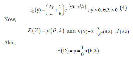
Also, for the generation of actual observed time y, we use the inverse cdf method which is given by:

Where, u is generated from U(0.1) Hence,

Maximum likelihood estimation

Let be a randomly censored sample drawn from the model in equation (2). Then, the likelihood function is given by

On putting and taking log on both sides, we get the log-likelihood function as given by

Therefore, the maximum likelihood estimation (MLE) of the parameters θ and λ are given by

Now, by using the second derivatives of the log-likelihood equation, we get the following Fisher information matrix as given below:

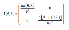
By inverting the diagonal terms of this Fisher information matrix, we get the variances of the parameters and after replacing the parametric values by their MLE’s, we can obtain the estimated values of the variances.

Also, two- sided equal tail 100x (1-α) % asymptotic confidence intervals for the parameters θ and λ are obtained as

Here, percentile of the standard normal distribution. The Monte Carlo simulation study can be performed to obtain the coverage probabilities (CP) as given by

Bootstrap confidence intervals

A parametric bootstrap interval provides much more information about the population value of the quantity of interest than does a point estimate. The parametric bootstrap methods are of two types:-

(i) Percentile bootstrap method (Boot-p) proposed by Efron [12].

(ii) Bootstrap-t method (Boot-t) proposed by Hall [13].

Percentile bootstrap method (Boot-p) confidence intervals

Step-1 A randomly censored sample is generated from the original data

of the parameter θ is computed.

Step-2 Again, an independent randomly censored bootstrap sample

Step-3 Now, compute the bootstrap MLE *ˆ θof parameter θ based on *x, as in step-1.

Step-4 Repeat steps 2-3, B times representing B bootstrap MLE’s *ˆ'_isθ based on B different bootstrap samples, i=1, 2,....B.

Step-5

boot-p confidence interval for θ is obtained by

Arrange all *ˆ'isθ in an ascending order to obtain the bootstrap sample i.e.

boot-p confidence interval for θ is obtained by

; where, [x] = integer part of x.

Bootstrap-t method (Boot-t) confidence intervals

Step-1 Steps 1 and 2 of boot-p and boot-t methods are same.

Step-2 Compute the bootstrap-t statistic

Step-3 To obtain a set of bootstrap statistics repeat steps 2-3, B times.

Now, the approximate 1001()%α×− boot-t confidence interval for parameter θ is obtained by

Expected time on test

Krishna et al. [10] developed the expected time on test for random censoring. In a life testing experiments, it is useful to have an idea about the expected duration of the experiment. In practical applications, it also helps in taking the number of items to be placed on test. Here, we deal with the mathematical formulation of expected time on test (ETT) with their maximum likelihood estimate and ratio of expected experiment time (REET) by considering a separate section of simulation to calculate the average values (AV) and the mean square errors (MSE) for different combinations of parametric values and sample sizes. In our case, Y be the healing or dropout time then we take the time on test as The cdf of Y(n) is given by

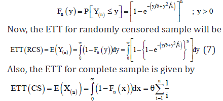
By applying the invariance property of MLE’s, we can obtain the estimated value of ETT. Note that, is the value of observed time on test (OBTT) in an observed sample i.e.

For comparing ETT, we compute the ratio of the expected experiment time (REET) for random censoring and the complete sample case i.e.

Bayes estimation

In Bayesian estimation of parameters, prior distributions for the unknown parameters θ and λ are incorporated with the likelihood function. Let the following independent inverted gamma priors for the parameters θ and ,λ which are assumed to be independent, are given by

The joint posterior distribution for the parameters are given by

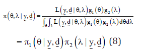
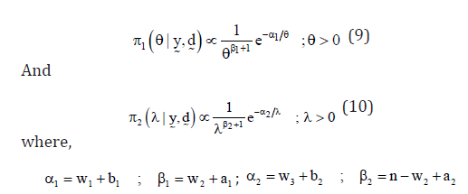
The marginal posterior distributions of the parameters θ and λ are given by

Generalized entropy loss function (GELF)

The GELF introduced by Calabria and Pulcini [14], is given by

The constant δ is its shape parameter which reflects the departure from symmetry. In the case, when δ< 0, under estimation by θ* of θ is considered to be more serious than over estimation of equal magnitude and vice-versa. The Bayes estimator of θ under GELF is given as

Note that in equation (11), if we put

• δ= -1, it provides the Bayes estimator under SELF.

• δ= 1, it gives Bayes estimates under ELF.

• δ= -2, it coincides with the Bayes estimates under PLF.

Therefore, the Bayes estimates for the parameters under GELF are given by

Sometimes, no prior information is available to us and then we use non-informative prior information. The Bayes estimates for non-informative priors can easily be obtained from the above expression by taking the hyper-parameter values

Antifungal resistance

Chen and Shao [15] introduced the following procedure to calculate highest posterior density (HPD) credible interval for the parameter θ. HPD credible interval has the shortest length among all credible intervals. First we generate 12,,...,Mθθθvalues from the posterior distribution and arrange these as ordered the integer part of x.

Also, for the parameter ,λ an HPD credible interval is obtained in the same manner. We use BOA package in software R for obtaining the HPD credible intervals.

Simulation study

For observing the behavior of the estimates, we deal with the simulation study in this section. Maximum likelihood and Bayes estimates under GELF are developed with confidence, bootstrap and HPD credible intervals. The step by step procedure is described below:

I. Choose different combinations for the parametric values of θ and λ with fixed sample size n=30.

II. Put the values of the hyper-parameters ()11,ab and ()22,abby taking 12aaa== and 12,bb equal to the means of prior distributions as ()111baθ=−and ()221.baλ=− For non-informative priors take 12120.

III. Generate a randomly censored sample ()y,d   of size n from the model in equations (4) and (1).

IV. Calculate the MLE’s for the parameters θ and λ with their asymptotic confidence intervals.

V. Bootstrap-p and t confidence intervals are also obtained by taking B=1000.

VI. Bayes estimates under GELF with associated HPD credible intervals for the parameters θ and λ are obtained with taking M=100.

VII. The average length (AL) and coverage probabilities (CP) for the asymptotic confidence and HPD credible intervals are also calculated.

VIII. For different combinations of the parametric values, repeat steps (iii-vi), N=1000 times. For each estimate obtained in step (iv-vi), the average value (AV) and mean square error (MSE) are computed.

Discussion on simulation study

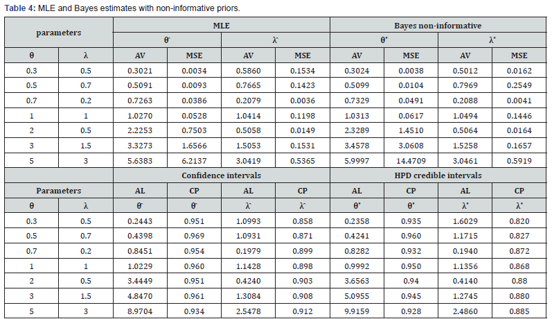
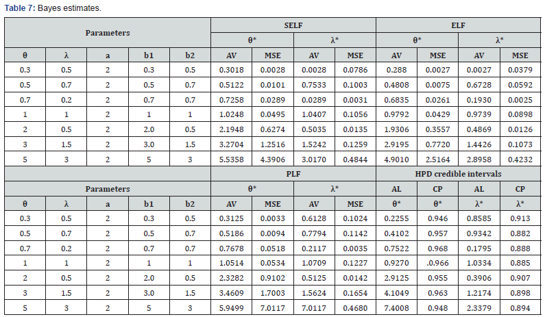
All the calculations were performed using the statistical software R. The main results of the simulation study are listed in tables 3-7 with these conclusions:

• Estimates obtained by maximum likelihood estimation are almost unbiased.

• Average Length of confidence intervals based on maximum likelihood estimation method increases as the parametric values increases and gives better coverage than the HPD credible intervals for non-informative priors.

• Bayes estimates under SELF also give very good results in respect of bias and MSE’s but Bayes estimates, for ELF show under estimation and for PLF show slight over estimation, in the estimation of parameters.

• HPD credible intervals using inverted gamma priors show a good coverage of probabilities than the asymptotic confidence intervals.

• Bootstrap confidence intervals give better coverage than the asymptotic confidence and HPD credible intervals in both boot-p and boot-t cases.

Real data example

In this section we analyze a real data set which consists of the survival times for 121 breast cancer patients treated over the period 1929-1938, quoted in Boag [16] and also given in Lawless [17]. Times are given in months and asterisks (*) denote the censoring times. The data set is given below:

0.3, 0.3*, 4*, 5, 5.6, 6.2, 6.3, 6.6, 6.8, 7.4*, 7.5, 8.4, 8.4, 10.3, 11.0, 11.8, 12.2, 12.3, 13.5, 14.4, 14.4, 14.8, 15.5*, 15.7, 16.2, 16.3, 16.5, 16.8, 17.2, 17.3, 17.5, 17.9, 19.8, 20.4, 20.9, 21, 21, 21.1, 23, 23.4*, 23.6, 24, 24, 27.9, 28.2, 29.1, 30, 31, 31, 32, 35, 35, 37*, 37*, 37*, 38, 38*, 38*, 39*, 39*, 40, 40*, 40*, 41, 41, 41*, 42, 43*, 43*, 43*, 44, 45*, 45*, 46*, 46*, 47*, 48, 49*, 51, 51, 51*, 52, 54, 55*, 56, 57*, 58*, 59*, 60, 60*, 60*, 61*, 62*, 65*, 65*, 67*, 67*, 68*, 69*, 78, 80, 83*, 88*, 89, 90, 93*, 96*, 103*, 105*, 109*, 109*, 111*, 115*, 117*, 125*, 126, 127*, 129*, 129*, 139*, 154*.

Now, first of all, we analyze the fitting of this real data set on two statistical models as exponential- Rayleigh and exponential-exponential. Maximum likelihood and Bayes estimation methods are applied for estimating the parameters of both the models. For goodness of fit experiment of the above models, we analyze

(i) Negative log-likelihood

(ii) Kolmogorov- Smirnov (K-S) test

(iii) Bayesian information criterion (BIC)

(iv) Akaike’s information criterion (AIC)

(v) Empirical cumulative distribution function (ECDF) curve.

Akaike information criterion (AIC)

AIC introduced by Akaike [18] under the name of “An information criterion”. The AIC is given by the following formula:

where k is the number of parameters and L is maximum likelihood function value for the estimated model.

Bayesian information criterion (BIC)

Bayesian information criterion, proposed by Schwarz [19], is a criterion for model selection among a class of parametric models with different numbers of parameters. It is very closely related to the AIC. The BIC is defined as:

Where k, n, L are same as in AIC. For this real data set, the values of goodness of fit experiments are shown below in Table 1.

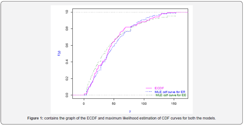
Figure 1 contains the graph of the ECDF and maximum likelihood estimation of cdf curves for both the models. From Figure 1, we observe that MLE cdf curve of our model is quite close to the ECDF curve. By all the above criteria of goodness of fit, we conclude that our model fits better than the exponential model. Now, these estimation methods are applied on this real data set for illustration purpose. The Estimates of the parameters derived as follows in Tables 2-7.

BBOAJ.MS.ID.555740

Our Media Partner

BBOAJ Menu

Useful Links

Downloads

References

- Friesl M, Hurt J (2007) On Bayesian estimation in an exponential distribution under random censorship. Kybernetika 43: 45-60.
- Abu-Taleb AA, Smadi MM, Alawneh AJ (2007) Bayes estimation of the lifetime parameters for the exponential distribution. Jour Math Stat 3: 106-108.
- Saleem M, Raza A (2011) On Bayesian analysis of the exponential survival time assuming the exponential censor time. Pak Jour Sci 63(1): 44-48.
- Ghitany ME (2001) A compound Rayleigh survival model and its application to randomly censored data. Stat. Papers 42(4): 437-450.
- Saleem M, Aslam M (2009) On Bayesian analysis of the Rayleigh survival time assuming the random censor time. Pak Jour Stat 25(2):71-82.
- Kim JH (1993) Chi-Square goodness-of-fit tests for randomly censored data. Ann Stat 21(3): 1621-1639.
- Ghitany ME, Al-Awadhi S (2002) Maximum likelihood estimation of Burr XII distribution parameters under random censoring. Jour App Stat 29(7): 955-965.
- Danish MY, Aslam M (2013) Bayesian estimation for randomly censored generalized exponential distribution under asymmetric loss functions. Jour App Stat 40(5): 1106-1119.
- Danish MY, Aslam M (2014) Bayesian inference for the randomly censored Weibull distribution. Jour Stat Comp Simul 84(1): 215-230.
- Krishna H, Vivekanand, Kumar K (2015) Estimation in Maxwell distribution with randomly censored data. Jour Stat Comp Simul 85(17): 3560-3578.
- Garg R, Dube M, Kumar K, Krishna H (2016) On Randomly Censored Generalized Inverted Exponential Distribution. Amer Jour Math Manag Sci 35(4): 361-379.
- Efron B (1982) The jacknife, the bootstrap and other re-sampling plans. CBMS-NSF Regional Conference Series in App Math Soc SIAM 38.
- Hall P (1988) Theoretical comparison of bootstrap confidence intervals. Ann Stat 16:327–953.
- Calabria R, Pulcini G (1996) Point estimation under asymmetric loss functions for left- truncated exponential samples. Comm Stat Th Meth 25: 585-600.
- Chen MH, Shao QM (1999) Monte Carlo estimation of Bayesian credible and HPD intervals. Jour Comp Graph Stat 8: 69-92.
- Boag, JW (1949) Maximum likelihood estimates of the proportion of patients cured by cancer therapy. Jour Roy Stat Soc B(11): 15-53.
- Lawless JF (2003) Statistical methods and models for lifetime data. John Wiley and Sons, New York.
- Akaike H (1974) A new look at the statistical model identification. IEEE Trans Autom Cont 19: 716-723.
- Schwarz G (1978) Estimating the dimension of a model. Ann Stat 6(2): 421–464.