Research Article

Bias Correction of Nonlinear Effect for Longitudinal Data

Yuanzhang Li*

Senior and Primary Statistician, George Washington University, USA

Submission: April 16, 2018; Published: October 24, 2018

*Corresponding author: Yuanzhang Li, PhD, Senior and Primary Statistician, George Washington University and Walter Reed Army Institute of Research, USA.

How to cite this article: Yuanzhang L. Bias Correction of Nonlinear Effect for Longitudinal Data. Biostat Biometrics Open Acc J. 2018; 8(3): 555739. DOI: 10.19080/BBOAJ.2018.08.555739

Abstract

Studying change from baseline measure in longitudinal data promises to lead to early identify a disease which would benefit both patients and society. The effect of antibody or biomarkers is certainly non-linear for human disease. Using longitudinal data and categorizing the first measurement may help to evaluate the non-linear effect, but it could confound the values of repeated measures and generate bias. We developed modeling strategies for case-control longitudinal studies to estimate and correct the bias. We use this approach in a military dataset to evaluate the association of antibody risk of developing schizophrenia. Cases and matched controls were grouped into categories by 50th and 75th percentile of the first sample of cases. The bias generated from such confounding is corrected by simulation to develop unbiased estimation. Seven antibody agents were studied. This proposed approach can aid investigators to identify risk factor in the pre-clinical period, and it can be extended to other longitudinal studies. Note: The views expressed are those of the authors and should not be construed to represent the positions of the Department of the Army or Department of Defense. None of the authors have any associations, financial or otherwise, that may present a conflict of interest.

Keywords: Bias correction; Longitudinal; Case control; Simulation; Confounding; Schizophrenia

Introduction

Case and control studies are commonly used in epidemiological research. When controls in a case-control study are not selected randomly from the population at risk, the effect estimates are likely to be biased. One of the bias is generated by confounding. Confounding mixes effect of a confounder - an extraneous factor in the study with the effect on predictor (exposure) on outcome that distorts the association between them. The observed relationship between exposure and outcome can be distorted totally or in part by the effect of the confounder. The analyses that involve longitudinal data generates biases due to data dependency and incompleteness. It is often that the effect of repeated measurements is temporal or non-linear. Categorize the baseline measurements often provides valuable information, when we are interested in the baseline assessment of specimen for the earlier identification effort with repeated measurements. It is clearly that the category of the first specimen is the confounder of the values of specimen and bias occurs, if the specimen risk on disease is compared between cases and controls.

In the literature, there are limited methods available to correct for the effects of biases on estimates of the exposure-disease relation. Recently, a simulation-based method of inference for parametric measurement error models in which the measurement error variance is known or at least well estimated was developed and studied [1-10]. The method entails adding additional measurement error in known increments to the data, computing estimates from the contaminated data, establishing a trend between these estimates and the variance of the added errors, and extrapolating this trend back to the case of no measurement error. In this study, we introduce a bias adjusted model by simulation.

Methods

Generalized linear mode is commonly used, with a large range of probability distributions that includes the normal, binomial and Poisson distributions, see Equation 1.

The logistic regression is a special case of generalized linear model, which is commonly used in the case-control study. As we discussed earlier, if confounder exists, the bias occurs. For the case-control study, our approach is to generate a set of simulated data with random assignment of cases and controls to perform the same analyses as that for the original data to estimate the bias. The general form of the model is

Where, X is a factor matrix, which generate unbiased estimations, Zis factor matrix, which includes all potential biased factors, γis the unbiased effect of Zon Y, δare the expected bias vector of the parameter estimation related to Z, σ is the variance of the bias ,δand ∈ is the random error. First, we use the simulated data to estimate the distribution of ,δand then use the original data to evaluate other parameters. We may estimate all unknown parameters simultaneously.

Application

Data for service members who received medical discharges with schizophrenia from 1992 to 2005 were obtained from the Physical Disability Agency (PDA) databases of the Army, Navy, Marines and Air Force. Those were cases. All control subjects were matched to their cases on sex (1:1 for male, 1:3 for female), race and age (within a year) and accession date (within a year). All serum specimens were obtained for cases. At least one, and up to four, matched specimens on the collection date within 90 days were selected for each control subject following four criteria:

1) The first available,

2) The most recent before diagnosis,

3) A middle between the two, and

4) The first available after the diagnosis.

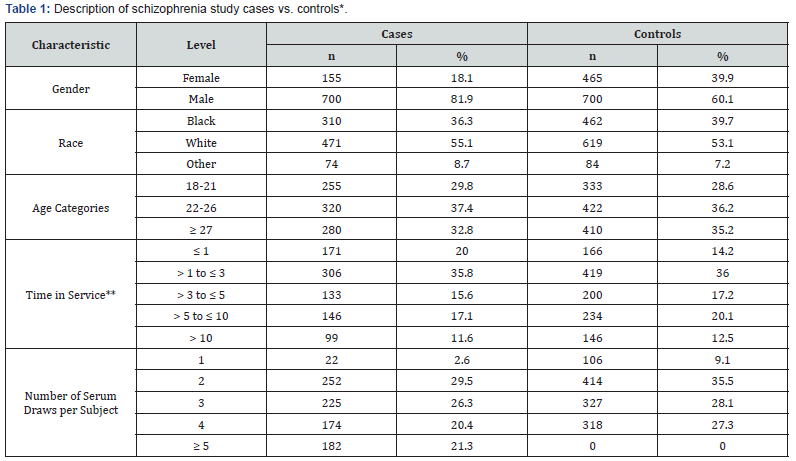
The food borne antigen casein was used in this study. We tested a total of 6106 serum samples from 855 cases and 1165 controls for schizophrenia. As shown in Table 1, the majority of cases were men, white, younger than 25 and had less than 3 years of service. Among the cases, fewer than 3% of patients had only one serum specimen available, about 30% had two and three, and approximately 40% had four or more specimens, which were collected up to 15 years before diagnosis as well as after diagnosis. Ninety-five percent of after-diagnosis specimens were collected within 1.8 years of the diagnosis. The association between agents and schizophrenia is examined, as well as the heterogeneity of the association by the agent baseline level and the time to diagnosis.

Hence the matched individuals (cases and controls) are categorized into three groups by their 50th and 75th percentiles of the first specimen of cases and examine the associations within one year before diagnosis and beyond one year before diagnosis. The conditional logistic regression was used. The outcome is the case (schizophrenia) status; the independent factors are subject group (categorized by the 1st specimen), the specimen collect time to diagnosis (one year before diagnosis, within one year to diagnosis), the agent level, their interactions, and the service time. The matched demographic factors are used as strata to control the heterogeneity of the standard error.

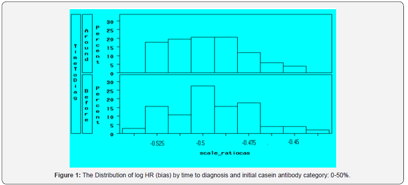
To correct the biases, 500 simulation data from the original data sets with randomly assigning case/control status are generated. Then the category of the 1st specimen was redefined according to the value of new data. Then simulation data is used to estimate the distribution of the modeling bias generated by confounding. Figure 1 shows the bias distribution of the scaled casein effect on those subjects with initial low level for different time period. It can be seen that both bias are negative with HR less than one. The mean of the biases were around -1, the distribution of the bias seems more flat than normal.

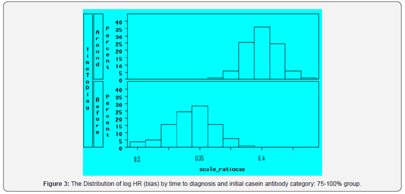
Figure 2 and Figure 3 show the bias distributions of scale casein for those subjects with initial higher levels. It can be seen the average bias increases as the initial value increasing. For those subjects with initial values higher than 75th percentiles, the bias distributions for the two time period were also different. Hence it is clear that the category of the 1st specimen is a confounder, which dramatically drives the estimation away from neutral. The bias of log of HR is far greater than zero.

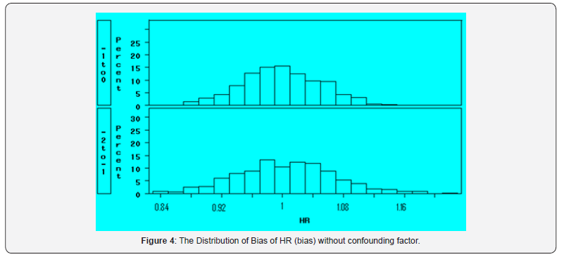
If excluding the confounder of the 1st specimen category from the modeling, the model includes the time period (after diagnosis, within one year before diagnosis, 1 to 2 years before diagnosis, beyond 2 years before diagnosis), specimen value, and the interaction, as well as other control factors. There is no obvious confounder in the modeling; Figure 4 shows the results the bias distribution from the same simulated data sets for the scale casein effect within one year to diagnosis and from 1-2 years before diagnosis. It can be seen that the distribution of HR are around 1.0.

It means the bias of log of HR is near 0. Then we perform the adjusting conational logistic model by suing simulation to estimate the bias δ and its distribution to the original data. We combine the two groups with higher initial values, both have positive confounding biases. Table 2 shows the parameter estimations of unadjusted parameter, the bias of the parameter and adjusted parameter as well as the related adjusted hazard ratios for one standard deviation of casein.

We can see that the category of the 1st specimen is still a confounder, which drives the estimation from neutral dramatically. However, after adjusting the bias, the associations between casein IgG antibody levels and the risk of schizophrenia exists for those who had higher initial level. The effect is also slightly different by the different time periods to diagnosis. For those, who had higher initial value, if their casein level increasing on standard deviation at one year pre-diagnosis, the risk to be schizophrenia increases about 12 percent (HR=1.12; 95% CI 1.07, 1.18). If we excluded the confounder of the 1st specimen category from the modeling, the model includes the time period (after diagnosis, within one year before diagnosis, 1 to 2 years before diagnosis, beyond 2 years before diagnosis), specimen value, and their interaction, as well as other control factors. There is no obvious confounder in the modeling; Table 3 shows the results from both unadjusted and adjusted models.

Discussion

The proposed approach in this study shows that the confounding bias could be adjusted by simulation. Confounding is a mixed effect of an extra factor that of interest predictor on outcome. It distorts the association between predictor and outcome. The observed relationship between the predictor and outcome can be attributed totally or in part to the effect of the confounder. Due to confounding, the model may overestimate or underestimate the true association between predictor and outcome; it could change the direction of the observed effect.

The proposed approach in this study can eliminated bias from confounding, if we know the confounder. However, before going to the adjusting model, it is very important to understand the data structure and the model design. The confounder should be correlated with both predictor and outcome. There are issues for the proposed approaches in this study should be further studied such as the bias distribution effect on the adjusting methods, the efficiency of the estimation methods, the number of simulations needed, the relation between the size of original data effect, etc. This paper mainly discusses the case-control studies, but it could be extended for other types of studies.

References

1. Allan J Rossman, Beth L Chance (2014) Using simulation‐based inference for learning introductory statistics. WIREs Computational Statistics 6(4): 211-221
2. Nathan Tintle (2001) Simulation-based inference in statistics education: Exciting progress and future directions.
3. Hardin JW, Carroll RJ (2003) Measurement Error, GLMs, and Notational Conventions. Stata Journal 3(4): 329-341.
4. Hardin JW, Carroll RJ (2003) Measurement Error, GLMs, and Notational Conventions. Stata Journal 3(4): 329-341.
5. Kleinbaum DG, Kupper LL, Morgenstern H (1982) Epidemiologic research: principles and quantitative methods. In: Belmont, CA: Lifetime Learning Publications, USA.
6. Last JM (1995) A dictionary of epidemiology. New York, NY: Oxford University Press, UK.
7. Hennekens CH, Buring JE (1987) Epidemiology in medicine. Boston, MA: Little, Brown and Company, USA.
8. Mallick R, Fung K, Krewski D (2002) Adjusting for measurement error in the Cox proportional hazards regression model. J Cancer Epidemiol Prev 7(4): 155-164.
9. Nordentoft M (2007) prevention of suicide and attempted suicide in Denmark. Epidemiological studies of suicide and intervention studies in selected risk groups. Dan Med Bull 54(4): 306-369.
10. Lee W, Bindman J, Ford T, Glozier N, Moran P, et al. (2007) Bias in psychiatric case-control studies. Br J Psychiatry 190: 204-209.