


Conditional Analysis and Unconditional Conclusion in Clinical Trial with Interim Analysis
Xi Chen*
PharmClint Co. Ardsley, USA
Submission: August 03, 2018; Published: October 04, 2018
*Corresponding author: Xi Chen, PharmClint Co. Ardsley, New York, USA; Email: xic001@gmail.com
How to cite this article: Xi Chen. Conditional Analysis and Unconditional Conclusion in Clinical Trial with Interim Analysis. Biostat Biometrics Open Acc J. 2018; 8(3): 555736. DOI: 10.19080/BBOAJ.2018.08.555736
Abstract
In the statistical analysis of a clinical trial with interim analysis, few of the currently existing methodology has ever presented a complete set of the assumptions and the rationale for these assumptions. The design of the trial with interim analysis is based on a conditional analysis, but the trial conclusion is completely unconditional. A linkage between the conditional analysis and the unconditional conclusion is mandatory for a complete set of the trial analysis. The purpose of this manuscript is to outline some basic research ideas against the current practice and the practical considerations which may lead to a feasible solution to this kind of analysis. The example shows that depends upon the algorithm for hypothesis tests, the error inflation caused by repeated significance test may not exist.
Keywords: Bayes’ analysis; Filtration; Interim analysis; Stochastic process
Abbrevations:PMF: probability mass function; SM: Study Medication; DF: Degree of Freedom;
Introduction
In a properly defined statistical analysis, the basic requirements include a complete specification of the sample space and a statistical model used in inference. The two are considered as key components for a statistical analysis, if there is any fuzzy description in the key components, the statistical analysis lost its foundation. For a clinical trial with interim analysis, although many techniques to deal with the error inflation caused by the repeated significance tests have been developed, the specifications of the key components were not complete, the clinical trial with interim analysis needs a further refinement.
A typical clinical trial design with interim analysis has been shown in Xia [1], a letter to the editor Chen [2] criticized the paper for failure to show the detail statistical model associated with the analysis. The rejoinder prepared by the original authors Xia [3] showed that the conditional probability was applied in the analysis. By default, a conditional statistical analysis can only reach a conditional statistical conclusion, but the claimed study medication efficacy in clinical trial is generally an unconditional statement. The relationship between the unconditional trial conclusion and the conditional statistical model was not explicitly specified.
The challenge can be understand in a more simple and straightforward way. A clinical trial is a scientific experiment, the experiment result or the trial conclusion has to be shown and interpreted through a scientific way. Consider a clinical trial with interim analysis as a stochastic process passing through a series of quality gates, for N processes started at the beginning of the trial, the number of the processes passing through all gates and reaching the final accept region can be expected. The claimed α value should be consistent to the ratio of this expected value to .N Any clinical trial design not able to layout such an outcome is subject to criticisms.
Consider the data accumulation in a clinical trial with interim analysis to be a stochastic process, there are three main purposes for this manuscript. The first is to clarify the sample space and the statistical model for a clinical trial analysis; the second is to clarify the relationship between the conditional analysis and the unconditional trial conclusion; the third is to show the process has to be ergodic and stationary.
As a significant discovery, the simulation result shows that the error inflation caused by the repeated significance tests is in doubt. In fact, the error inflation is related to the algorithm for the hypothesis test and the parameter estimation. In practice, the error spending philosophy presented in Lan [4] is widely used without a detailed discussion of the hypothesis test algorithm, such a practice may have a negative impact on the confidence of the hypothesis test.
Current Clinical Trial Practices
Setup of the sample space
It is noted that based on the setup of the sample space, a clinical trial with interim analysis can be interpreted in differentways, which may lead to different statistical models. Obviously, the random samples for different trial stages will fall on different subsets of the full sample space, if the sample space is assumed to be unchanged, the analysis for each stage can only be a conditional analysis.
The problem of Xia [1] is that it did not explicitly define the sample space in the clinical trial with interim analysis. The rejoinder Xia [3] claimed that the sample space Ω to be a K dimensional discrete space, with K orthogonal axes. The fundamental question is on the statistical model defined on such a space, and how to derive the trial conclusion in such a sample space. More specifically, the algorithm of 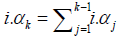 will be questionable. If i.αj are evaluated with respect to different axes of a Cartesian coordinate system, the summation should be understand as an operation in a vector space, not the simple arithmetic summation.
One of the most important tasks for this manuscript is to show that the sample space for the trial with interim analysis will remain same as Ω which could not be the multiple dimensional. Any statistical inference is with respect to Ω and the fixed statistical measure .P Without such an explicit setup of the analysis foundation, the type I error referred in Xia [1] does not have a basic support. In the other words, it needs an explanation how does αbe interpreted.
Conditional analysis and unconditional conclusion
When performing a conditional analysis, most of the estimations are in fact the conditional estimations. For example, within a census database, if the mean age of the female subjects is estimated, the output will be the mean age of the female population. Obviously, the mean age of the female population can be different from that of the general population, but the definition of the mean remains the same.
Return to the clinical trial with interim analysis, at the final stage of the trial, only the samples passed the (1)kth interim gate can be observed. It is for sure a conditional estimate, how can this estimate be interpreted as the unconditional conclusion depends upon the trial setup. Obviously, upto this point, such a setup is not obvious in available literature.
Basic assumptions
In a clinical trial analysis, assume the data accumulation forms a stochastic process, with or without any interim analysis, the process has to be ergodic and stationary, see Walters [5]. For ergodicity, it implies that the process averages over the time will be the same as it averages over the sample space, so the estimation accuracy can be improved through the prolongation of the process observation. For stationary, it implies that the statistical model remains the same over the time, any statistical conclusion is regarding to a unchanged statistical model. Besides, a proper statistical analysis requires the sample space remains the same over the time.
If these assumptions are met in the clinical trial design have to be declared explicitly in the protocol or the statistical analysis plan, they serve as the pre-requisites for the statistical analysis. If it is necessary, the properties have to be shown. If the proof is impossible, the assumptions have to be shown in trial set up, and the assumptions could not be violated during the trial progress.
On the other hand, for a clinical trial with interim analysis, if there is an error in inflation caused by the repeated significance tests, the error inflation should be intrinsic. In the other words, the error inflation may depend upon the estimation algorithm, the algorithm which causes the smallest error inflation should be applied
Error inflation and its elimination
The error inflation caused by the repeated significance test is a well known phenomenon, for example, see Bonferroni [6]. But unfortunately, such a phenomenon is just an observation in practice, its existence has never been mathematically proved. The observed error inflation may be caused by the estimation algorithm for the test, different algorithms for estimation may lead to different error inflation rate. For example, Anscombe [7] has observed that the inference through the likelihood maybe unaffected. The techniques to deal with the error inflation caused by the repeated significance tests also have many problems. For example, Armitage [8] has developed a quadrature to deal with the error inflation,

The problem is that no matter what specific ()fx is chosen, nf and 1nf− cannot remain as a same distribution. In the sense, the process ()fx is not stationary, it does not meet the basic assumption to the trial setup.
The α spending methodology developed by Lan [4] used the similar quadrature in derivation, and the work of Xia [1] followed the same pattern un-explicitly. It is noted that both works did not discuss the estimation algorithm into detail, but the error inflation is sensitive to the algorithm. In the sense, without an extensive validity discussion regarding the spending, along with a different estimation algorithm, different αspending methodologies can be applicable, which may lead to a different statistical conclusion.
More criticisms on Xia’s formulation
The statistical model presented in Xia [1] is
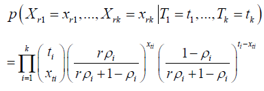
The validation of this statistical model is in questions. The complete specification of the statistical model has to present what is the information which can be directly observed from the data, and what are the parameters to be estimated. For the parameters to be estimated, the complete specification has to outline the model and the algorithm for parameter estimation, since different models will lead to different ways in the estimation. More specifically, if r is a parameter has to be specified in the manuscript.
In Xia [1], for either case of r=1 or r=0.5,r is considered as a constant not a parameter. In the case, the hypothesis H0:r=1 vs. H1:r< 1 is ill-fated since the hypothesis assumes r to be a statistic and the test of the hypothesis depends upon the estimation of .r If ris a parameter, without a complete algorithm to estimate ,r the above model specification is incomplete. To understand the challenge in a more clear arguments, both cases r=1 or r=0.5 do not provide the information regarding the case r=0.7 or r=0.8 a natural question is that when r=0.7 or r=0.8, what kind of the trial outputs will be observed.
Besides, Xia [3] stated that “ we assume equal allocation of person years into the vaccinated and placebo groups at each stage ()1230.5ρρρ=== as is typically done. But as shown in Section 3 our methods are robust to non-equal allocations and non-constant proportions.” The statement is not true, since whenkρ changes over ,k the process is no longer stationary, it is against the basic requirements for the analysis. Finally, the derivation of the “adjusted futility safety” boundary has not been described in detail, based on the information given by the manuscript, it is impossible to reproduce the result in the Table 1 of Xia [3].

Moreover, there are still some other challenges to the setup of the statistical model. Among them, the efficacy of the study medication is generally characterized by a unconditional statistical characteristic since the claim of the efficacy is generally an unconditional statement. The relationship between the unconditional conclusion and the above conditional statistical model has to be clarified. The conditional probability mass function (PMF) presented in the manuscript is a function of 1,...,,ktt in the other words, it implies that for a different set of 1,...,kTT values, saying 1,...,,kττ the conditional PMF will be different. It is against the basic definition of the study medication efficacy. The efficacy of the study medication is a unconditional measure which implies the efficacy of the study medication does not depends upon the conditions in which the clinical trial is performed. When a conditional probability model is used, it is necessary to establish the relationship between the conditional analysis and the unconditional conclusion. Without such a relationship, the conclusion of the clinical trial with interim analysis is not convincing.
Statistics Fundamentals
These statistics fundamentals are essential to the conditional probability analysis, they basically explained why the unconditional estimations can be obtained from the conditional analysis.
Sample space and measure
In statistical analysis, a σ-field (or aσ algebra) on a set Ω is a collection F of subsets of Ω that includes the empty subset, is closed under complement, and is closed under union or intersection of countably infinite subsets. The pair (Ω,F) is called a measurable space. There are three key motivators forσ -field, defining measures, manipulating limits of sets, and managing partial information.
To perform a statistical analysis, a measure P is defined in the measurable space. For a clinical trial analysis, it is assumed that the statistical model across different stages to remain the same, so the measureP will not change over stages. The triplet (),,FPΩ forms a probability space.2,FΩ⊂ where 2Ω is its power set which contains all the subsets of ,Ω is aσ-algebra.
For limits of sets, if F1,F2,F3,.. are in ,F the  More importantly,
When only partial information can be characterized with a smaller σ-algebra which is a subset of the principalσalgebra, it is considered as a sub σ-algebra. In our notation, the principal σ -algebra is ,F any kFF⊂ is a sub σ-algebra.
It is important to see that based on this set up, the unchanged P and Ω secured the requirements that the process to be stationary and the consistency of the sample space throughout the analysis.
Filtration
In the setup of the probability space (),,,
I. A σ-field (),FΩ consists of a sample space Ω and a collection of subsets F satisfying the following conditions :
• Contains the empty set ()F∅∈.
• Is closed under complement ()cEFEF∈→∈.
II.
Given the σ-field (),FΩ with 2,FΩ= a filtration is a nested sequence 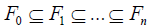 of subsets of 2Ω such that:
• ()0,Fθ=Ω (no information).
• 2nFΩ= (full information).
• For ,inθ≤≤ (),iFΩ is a σ-field (partial information).
III. Essentially a filter is a sequence of σ-field such that each new σ-field corresponds to the additional information that becomes available at each step and thus the further refinement of the sample space .Ω
It should be noted that the filtration with the second property is also called non-anticipating, i.e., one cannot see into the future. At the kth stage of the clinical trial with interim analysis, the trial sponsor cannot arbitrarily assume the clinical outcome beyond the stage, the maximum prediction of the trial outcome beyond the kth stage is based on the data accumulation up to the kthstage. In fact, any prediction to the process beyond the kth stage is against the nature of the clinical trial goals.
Conditional distribution and Bayes formula
Let ()PA refers to the probability of A and P(B) as that of .B P(A|B) refers to the probability of
A given that B happens. With the Venn diagrams, it is straightforward to see that P(A|B)
Through the Bayes formula, we can rewrite that equation as 
It is important to understand the relationship  outlined in the definition of the filtration correctly. The subset relationship is under the meaning of the set theory, not the simple interval concept on real axis. For example,
  and ()0.5,1,kF= then 1.kkFF+⊆ On the other hand, if ()10.3,1,kF+= kF is not a subset of 1,kF+ although in conventional analysis, (0.5,1) can be considered as a segment of (0.3,1), it is not under the sense of set theory. More interestingly, when evaluate
  the information of kF is mandatory, ()1PrkkFF+∩ provides new information brought by 1kF+ for the intersection.
Filtration and the foundation for analysis
Any statistical analysis has to be built upon a uniquely defined statistical distribution, .P It is crucial to realize that for an event in ,Ω say ,E along with a filtration ,iF an estimation can be in the form of either ()PE or (|),iPEF but both of them are mathematical characteristics of .P Assume that the estimates are means of a distribution, say ,μ obviously ()()iEEFμμ≠ in general. But, there are two things to be secured. First, both sμ are measured by same ;P second, the relationship between ()Eμ and ()iEFμ has to be specified. The problem of Xia [3] is that it did not specify such a relationship explicitly, so his trial design is not convincing. In a clinical trial analysis, the results in subgroup analysis can only be considered as observational, they could not be a confirmative conclusion. It more or reflects such a logic, but it generally did not give the reasons explicitly.
The relationship between ()Eμ and ()iEFμ within our framework will be shown in later sections along with the definition of the filtration. It is in fact the key for this manuscript.
Clinical Trial with Interim Analysis
Filtration associated with interim analysis
It has been shown that throughout the clinical trial with interim analysis, the sample space Ω and the statistical model Premain unchanged, the statistical inference at all stages are with respect to Ω and .
Assume the statistical inference is based on the likelihood ratio test, which will be discussed into the detail in the following section, the test statistics will be 1,...,..,..,kKλλλ The filtration with respect to Ω could be
• 0F is the trivial σ-field
• 1F consists of all the processes passing the first interim gate
•
• 1KF− consists of all the processes passing the final interim gate,
• KFconsists of all the processes reach the accept region at the end of the trial.
Clinical trial with interim analysis
The study hypothesis is setup same as that in Chen [9],
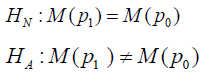
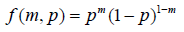
Where M(p1) is the statistical model to characterize the study medication (SM) and M(p1) is the statistical model to characterize the comparator (AC). Different from the conventional analysis, no matter the null hypothesis or the alternative hypothesis to be true or false, the statistical model for inference,  remains the same. The probability mass function (p.m.f.) can be written as
 consider the joint distribution of SM and AC arms, two statistical model
 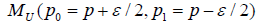 with likelihood UL and
 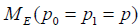 with likelihood EL are compared.
Lett 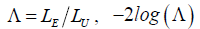 is
is  distributed with degrees of freedom of 1. Under the distribution assumption, with
 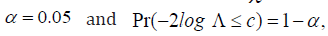 it can be shown that 3.84.c= It implies that when
 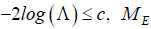 is considered to be the correct model; otherwise, the correct model is .UM It is noticed that this likelihood ratio analysis is applicable to a trial without interim analysis, and it is also applicable to each stage in the trial with interim analysis.
For a trial with interim analysis, it is noticed that let 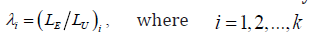 represents the stage,
 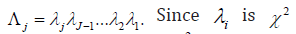 distributed with degrees of freedom of 1 is χ2 distributed with degrees of freedom of .j
When the trial is executed along with the interim analysis, at the stage ,k the test is performed on kΛ conditional on 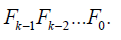
Trial inference
It is noted that 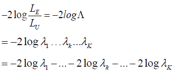
where the subscript k represent the kth interim analysis during the trial, 2logkλ− is χ2 random variable with degree of freedom (df) of 1 for 1,2,...,,kK= then 12logkjjλ=−Σ is χ2 distributed with dfk= then 2 log−Λ is χ2 distributed with degree of freedom of .K Note that 12logkjjλ=−Σ can be calculated at the kth interim gate based on the cumulated data up to that time point.
Consider the statistical inference of the problem at each stage, 1,2,,,
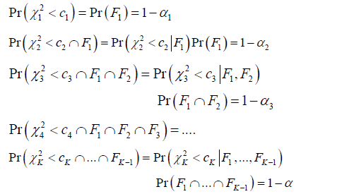
Where 2kkcχ< implies the test statistic 212log...kkχλλ=− is a χ2 statistic with dfk= and kc is the critical value derived from
In the analysis, let 1N be the number of the processes reached the accept region in the first interim gate, so 1-α can be estimated by 1.NN Immediately after the first interim gate, ()()212PrKFcχ< can be estimated by 12NN where 2N is the number of the processes passing the first interim gate and reached the accept region at the second interim gate, and ()1PrF can be estimated by 1.NN Combining them together, it shows that 2-α can be estimated by 12.NN With same inference, from the last equation, it is known that ()11PrKFF−∩ can be estimated by 1,KNN− where 1KN− is the number of the processes passing the (k-1)th interim date, and N is the number of the processes started at time 0. ()()211Pr,...,KKKcFFχ−< can be estimated by 1,KNN− where kN is the number of the processes ended up in the accept region, it is easy to see that 1-α can be estimated byNN
It should be noted that during the inference, two of the fundamental assumptions have been made. First, all the process falls in the accept region at the (k-1)th interim gate will automatically proceed to the kth stage, and all process falls in the rejection region at the(k-1)th interim gate will be terminated. Second, the ergodic property is mandatory, so the KNN can be the estimate for -α In theory, -α refers to the probability of the samples from one process fall in accept region over the time, but KNN refers to the result of multiple processes at a specific time point .KThe ergodicity property guarantee that the sample over time and the sample over sample space will remain the same.
Rationale of the trial design
Return the discussion started in section 3.4, the above analysis provides a rationale to link the observation to the trial goal. More specifically, at the Kth stage of the trial, only ()()211Pr,...,KKKcFFχ− =
=  the trial design itself will have problem. In the sense, the above analysis is by no means redundant, it serves a key role to link the conditional analysis with the unconditional statistical conclusion.
Another important finding through the analysis is that the continuation rule and stop rule implied by the trial design are strict, any trial execution in violation to the rules will destroy the integrity of the trial. Although multiple violations may compensate each other, the strict quantification might be difficult. Besides, the concepts such as adjusted futility safety boundary or adjusted efficacy boundary are no longer necessary, since the likelihood ratio test is based on different test statistics compared with the conventional analysis.
It is noted that the above analysis is not a strict proof of =the strict proof related to the property of 11....KFF−∩∩ In fact, such a proof is related to the existence of the error inflation caused by the repeated significance tests. Our proof can be considered as a weak proof, since it at least showed that both and unconditional can be estimated by the same test statistics, Nk/N
Example
As an example, a simulation is performed with the pseudo random number generator. The outcomes of SM and AC follow the Bernoulli distribution with same cure rate 0.5,p= so the efficacies of the SM and AC are the same. It is assumed that 0.05α= which remain the same over the stages, there are 4 interim analyses with even space. As result, kα and corresponding critical values kcare distributed as in Table 1.
For 2,k= 20.05,α= 25.99c= is derived from ()220.05,χ which represent the χ2 distribution with degree of freedom 2. In each simulation run, 1000 pairs of SM and AC efficacy samples were created, and the interim gates were placed with even space over the 1000 pairs. The simulation is run 1,000 times, the number of the processes passing each of the interim gates, ,kN are summarized.
The simulation show that among 1000 trial processes, at the first interim date, 950 trials concluded that the SM performed same as AC. The result is consistent to the presumption that α=0.05 For the following interim gates, the difference between the observed 5943N=with the theoretically expectation of 5950N= was due to the random error since the sample size is limited.
This simulation did not explicitly deal with the error inflation, but since the likelihood ratio test is used in statistical inference, the error inflation caused by the repeated significance tests has not been obviously observed. Besides, the likelihood ratio test is based on the mean of the random variables, not the lower or upper bound of the confidence interval, so the methodology of the spending is not used, the adjustment for the error inflation may not be necessary.
Discussion
Interpretation of the confidence
In any clinical trial design, a confidence level is claimed. But, within the trial setup of Xia [3] (2007), the foundation of is not clear. Specifically, a cited value has to associated with a sample space and a chosen statistical model. Within a conditional analysis, the independence of to the trial execution conditions has not been explicitly shown. If the trial execution conditions have impacts on the value, the trial conclusion will be in question.
In our setup of the clinical trial, the α is always measured by P on the foundation of Ω which remain unchanged throughout the trial. More specifically, α estimation is independent to the filtration 11,...,,KFF−so the trial conclusion is completely unconditional
A debate may arise since it is shown that -α can be estimated by ,KNN but since at the time point K ,Kαα= KNdoes not depends upon any of the previous interim gate criteria, so KNN is independent to all the interim gates. In fact, KN is not completely independent to kN for ,kK< since obviously, we have KkNN< for all ,kK< the trial stopped at any interim gate could not proceed to the final quality gate. The analysis showed that estimation across the sequence of the interim gates form a Markov chain. it will not be discussed into the detail and the door for further study remains open.
Distribution assumptions
In this manuscript, the binomial distribution is assumed. The same logic is also applicable to the statistical analysis based on Poisson model as well as the other statistical models. The rejoinder, Xia [3], disqualified the binomial model for the foundation that the comparative Poisson model dealt with the lower probability rate. But, the probability rate of the Poisson model is not discussed into the detail. In fact, if the understanding of the presented Poisson model is correct, the probability rate of the Poisson model is ,iρ which is assumed to be 0:5 which is close to the probability rate 0.5p= in this binomial set up.
The key argument is that for any distribution assumptions, the clarification of the parameters and the estimation algorithm for the parameter estimation are mandatory for the model specification. The maximum likelihood estimates should be adopted, and the statistical inference should be based on the likelihood ratio test. The error inflation caused by the repeated significance tests may not exist. Naturally, this manuscript could not be considered as a theoretical proof that the likelihood ratio test completely eliminated the error inflation in practice, the topic still remains for further discussion.
Main contributions
The main purpose of this manuscript is to show that no matter with a conditional analysis or a unconditional analysis, the statistical analysis of a clinical trial data is regarding to a fixed P and ,Ω the trial conclusion should always be unconditional. In the other words, the trial conclusion is always independent to the conditions in which the trial was executed. On the other hand, consider the trial data accumulation form a stochastic process, the process has to be ergodic and stationary. If these properties were not secured, any trial conclusion will not be on a solid statistical foundation.
References
- Xia Q, Hoover D (2007) A Procedure for Group Sequential Comparative Poisson Trials. J Biopharm Stat 17(5): 869-881.
- Chen X (2017) Letter to the Editor on A Procedure for Group Sequential Comparative Poisson Trials by Xia and Hoove. J Biopharm Stat 27(1): 186-190.
- Xia Q, Hoover D (2017) Rejoinder to Chen’s letter. J Biopharm Stat 27(1): 191-193.
- Lan KKG, DeMits DI (1983) Discrete sequential boundaries for clinical trials. Biometrika 70(3): 659-663.
- Walters P (1982) An introduction to ergodic theory. Graduate Texts in Mathematics, Springer-Verlag, UK.
- Bonferroni C (1936) Teroria statustuca della classi e calcolo delle probabilita. Pubblicazioni del R Istituto Superiore di Scienze Econommiche e Commerciali di Firenze 8: 3-62.
- Anscombe FJ (1954) Fixed sample size analysis of sequential observations. Biometrics 10: 89-100.
- Armitage P, McPherson CK, Rowe BC (1969) Repeated significance tests on accumulating data. JR Statist Soc A 132(2): 235-244.
- Chen X (2013) A non-inferiority trial design without need for a conventional margin. Journal of Mathematics and System Science 3: 47-54.


