


A New Flexible Distribution Based on the Zero Truncated Poisson Distribution: Mathematical Properties and Applications to Lifetime Data
Abouelmagd THM*
Management Information System Department, University, Saudi Arabia
Department of Statistics, Mathematics and Insurance, Benha University, Egypt
Submission: June 13, 2018; Published: August 14, 2018
*Corresponding author: Abouelmagd THM, Department of Statistics, Mathematics and Insurance, Benha University, Egypt, Management Information System Department, Taibah, University, Saudi Arabia; Email: tabouelmagd@taibahu.edu.sa
How to cite this article: Abouelmagd THM. A New Flexible Distribution Based on the Zero Truncated Poisson Distribution: Mathematical Properties and Applications to Lifetime Data. Biostat Biometrics Open Acc J. 2018; 8(1): 555729. DOI: 10.19080/BBOAJ.2018.08.555729
Abstract
In this paper, we introduce a new three-parameter model based on the zero truncated Poisson lifetime model. The new model has a strong physical motivation. We provide a comprehensive treatment of its statistical properties including ordinary and incomplete moments, generating functions and order statistics. The method of maximum likelihood is used to estimate the model parameters. We prove empirically the importance and flexibility of the new model in modeling two types of lifetime data.
Keywords: Zero truncated poison; Order statistics; Maximum likelihood estimation; Generating function; Moments
Abbrevations: ZTP: Zero Truncated Poisson; RV: Random Variable; PMF: Probability Mass Function; CDF: Cumulative Distribution Function; PDF: Probability Density Function; TLW: Topp Leone Weibull; ZTPTLW: Zero Truncated Poisson Topp Leone Weibull; PWMs: Probability Weighted Moments; RS: Random Sample; MLE: Maximum Likelihood Estimation; GaEE: Gamma Exponentiated Exponential; EEGc: Exponential-Exponential Geometric; PMF: Probability Mass Function
Introduction and Motivation
The so called zero truncated Poisson (ZTP) distribution is a discrete probability model whose support is the set of only the positive integers ()+I. The ZTP is also known as the positive Poisson distribution or the conditional Poisson distribution. It is the conditional probability distribution of a Poisson-distributed random variable (RV), given that the value of the RV is 0.≠ Thus, it is impossible for a ZTP RV to be zero, in this paper we will introduce a new flexible model based on the ZTP distribution for modeling lifetime data.
Suppose that a system (machine) has N subsystems functioning independently at a given time where N has ZTP distribution with parameter .λIt is the conditional probability distribution of a Poisson-distributed random variable, given that the value of the random variable is not zero. The probability mass function (PMF) of N is given by

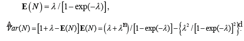
Note that for ZTP variable the expected value ()()NEand variance ()()VarNare, respectively, given by
Due to Rezaei et al. [1], the cumulative distribution function (CDF) and the probability density function (PDF) of the Topp Leone Weibull (TLW) distribution specified by

respectively. Suppose that the failure time of each subsystem has the TLW model defined by CDF and PDF in (2) and (3). Let iY denote the failure time of the i(th)sub system and let

Therefore, the marginal CDF of X is can be expressed as

Equation (5) is called the CDF of the zero truncated Poisson Topp Leone Weibull (ZTPTLW) model. The corresponding PDF of (5) reduces to

Now we can provide a useful linear representation for the ZTPTLW density function in (6). Expanding the quantity A in power series, we can write

Consider the power series

using the power series in (8) and after some algebra the PDF of the ZTPTLW in (7) can be expressed as

Equation (9) reveals that the density of X can be expressed as a linear representation of exponentiated-W (Exp-W) density. By integrating (9), we have

is the CDF of the Exp-W odel with power parameter .γ Some generalization of the Weibull distribution studied in the literature includes, but are not limited to Yousof et al.[2], Afify et al. [3,4], Alizadeh et al. [5], Yousof et al. [6-9], Brito et al. [10], Cordeiro et al. [11,12], Aryal & Yousof [13], Korkmaz et al. [14,15], Yousof et al. [16-19], and Hamedani et al. [20], among others The ZTPTLW model is very attractive to introduce sub-models with different types of the hazard rates. Figure 1(a) displays some plots of the ZTPTLW density for different values of ,λ α and .b These plots reveal that the ZTPTLW density can be right-skewed model. The HRF plots of the ZTPTLW distribution given in Figure 1(b) can be unimodal, bathtub, increasing and decreasing shapes.
The justification for the wide practicality of the ZTPTLW lifetime model is based on the wider use of the W model, as well as we are motivated to introduce the ZTPTLW lifetime model because it exhibits the unimodal, the bathtub, the increasing and the decreasing hazard rates as illustrated in Figure 1(b). It is shown in above that the ZTPTLW lifetime model can be viewed as a mixture of the Exp-W distributions. It can be viewed as a suitable model for fitting the unimodal and right skewed data. The proposed ZTPTLW lifetime model is much better than the Marshall Olkin extended W, gamma W, W Fréchet, Kumaraswamy W , beta W, transmuted modified W, Kumaraswamy transmuted W, modified beta W, the Mcdonald W and transmuted exponentiated generalized W models so the ZTPTLW lifetime model is a good alternative to these models in modeling aircraft windshield data as well as the new lifetime ZTPTLW model is much better than the WW, odd WW, W Log W, the gamma exponentiated-exponential and exponential-exponential geometric models so the ZTPTLW lifetime model is a good alternative to these models in modeling the survival times Guinea pigs.

Mathematical properties
Probability weighted moments (PWMs)
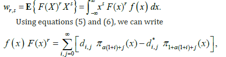
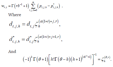
The (s,r)th PWMs of X following the ZTPTLW is defined by
Moments, incomplete moments and generating function
The ()thr ordinary moment of X is given by 

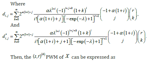
Where 
The ()ths incomplete moment, say (),stτ of Xcan be expressed from (9) as
The moment generating function (MGF) ()()()expXMttX=E of X can be derived from equation (9) as
Residual life and reversed residual life functions
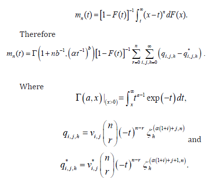
The ()thnmoment of the residual life is given by 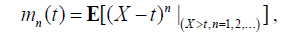
the ()thnmoment of the residual life of X is given by
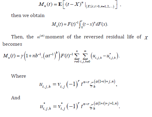
The ()thnmoment of the reversed residual life, say
Order statistics
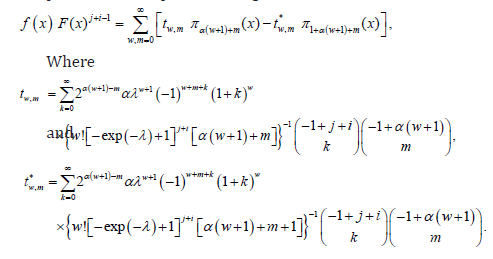
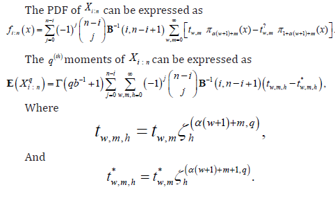
Let X1,...,Xn be a random sample (RS) from the ZTPTLW distribution and let X1:n,...,Xn:nthe corresponding order statistics. The PDF of the i(th)order statistic, say :,inXcan be written as

where B(⋅,⋅) is the beta function. Substituting (5) and (6) in equation (13) and using a
power series expansion, we get
Estimation
Let X1,...,Xnbe a random sample(RS) from the ZTPTLW model with parameters ,,aλαand .b Let (),,TbλαΨ= be the 31×parameter vector. For determining the maximum likelihood estimation (MLE) of Ψ, we have the log-likelihood function
. 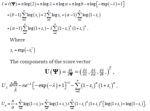
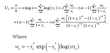
Via setting the nonlinear system of equations Uλ=Uα=0and Ub=0 and the solving them simultaneously yields the 
Applications
In this section, we provide two applications of the ZTPTLW model to show empirically its potentiality. In order to compare the fits of the ZTPTLW model with other competing distributions, we consider the Cramér-von Mises (W*)and the Anderson-Darling (A*) statistics. The two statistics are widely used to determine how closely a specific CDF fits the empirical distribution of a given data set. These statistics are given by
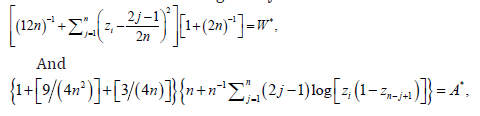
respectively, where Zi=F(yj) and the yj’s values are the ordered observations. The smaller these statistics are, the better the fit. The required computations are carried out using the R software. The MLEs and the corresponding standard errors (in parentheses) of the model parameters are given in Tables 1 and 2. The numerical values of the statistics W* and A* are listed in the same Tables. The histograms of the two data sets and the estimated PDF of the proposed model are displayed in Figures 2 & 3.


Failure times
The data consist of 84 observations. Here, we will compare the fits of the ZTPTLW distribution with those of other competitive ones, namely: the gamma W (GaW) [21], the Marshall Olkin extended W (MOEW), the W Fréchet (WFr) [4], the Kumaraswamy W (KwW) [22], the transmuted modified W (TMW) [23], the beta W (BW) (Lee et al., 2007)[24], the modified beta W (MBW) [25], the Kumaraswamy transmuted W (KwTW), the Mcdonald W (McW) [26], and the transmuted exponentiated generalized W (TExGW) models, whose PDFs are given by:

The parameters of the above densities are all positive real numbers except for the TMW and TexGW distributions for which 1.λ≤ Tables 2 list the values of above statistics for seven fitted models. The MLEs and their corresponding standard errors (Ses) (in parentheses) of the model parameters are also given in these tables. The figures in Table 1 reveal that the ZTPTLW distribution yields the lowest values of these statistics and then provides the best fit to the two data sets.
Survival times
The second real data set corresponds to the survival times (in days) of 72 guinea pigs infected with virulent tubercle bacilli reported by Bjerkedal [27]. We shall compare the fits of the ZTPTLW distribution with those of other competitive models, namely: odd WW (OWW) [28], WW, the gamma exponentiated exponential (GaEE) [29], W Log W (WLogW) [30], and exponential-exponential geometric (EEGc) [31], distributions, whose PDFs are: given by
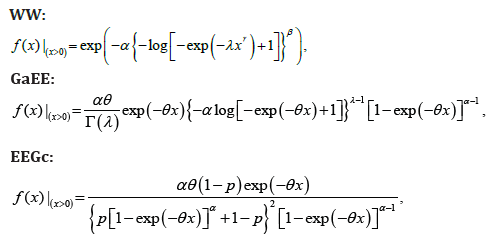
Based on the figures in Tables 1 & 2 we conclude that the ZTPTLW lifetime model provide adequate fits as compared to other Weibull-G models in both applications with small values for *W and *.AIn Application 1, the proposed ZTPTLW lifetime model is much better than the MOEW, GaW, KwW, WFr, BW, TMW, KwTW, MBW, McW, TExGW models, and a good alternative to these models. In Application 2, the proposed ZTPTLW lifetime model is much better than the WW, OWW, WLogW, GaEE, EEGc models, and a good alternative to these models [32,33].
Conclusion
In this paper, we introduce a new three-parameter zero truncated Poisson lifetime model. We provide a comprehensive account of some of its statistical properties including ordinary and incomplete moments, generating functions and order statistics. The maximum likelihood method is used to estimate the model parameters. We prove empirically the importance and flexibility of the new model in modeling two types of lifetime data. The proposed ZTPTLW lifetime model is much better than the Marshall Olkin extended Weibull, Kumaraswamy transmuted Weibull, Kumaraswamy Weibull, Weibull Fréchet, beta Weibull, gamma Weibull , transmuted modified Weibull, modified beta Weibull, Mcdonald Weibull and transmuted exponentiated generalized Weibull models so the ZTPTLW lifetime model is a good alternative to these models in modeling aircraft windshield data as well as the new lifetime ZTPTLW model is much better than the odd Weibull, Weibull Log Weibull, Weibull, the gamma exponentiated-exponential and exponential-exponential geometric models so the ZTPTLW lifetime model is a good alternative to these models in modeling the survival times Guinea pigs. We hope that the new distribution will attract wider applications in reliability, engineering and other areas of research.
References
- James G, Witten D, Hastie T, Tibshirani R (2013) An Introduction to Statistical Learning, Springer, New York.
- Zweig MH, Campbell G (1993) Receiver-operating characteristic (ROC) plots: a fundamental evaluation tool in clinical medicine. Clin Chem 39(4): 561-577.
- Fawcett T (2006) An Introduction to ROC Analysis. Pattern Recognition Letters 27(8): 861-874.
- Baker S (2003) The Central Role of Receiver Operating Characteristic (ROC) Curves in Evaluating Tests for the Early Detection of Cancer. Journal of the National Cancer Institute 95: 511-515.
- Youden WJ (1950) Index for Rating Diagnostic Tests. Cancer 3(1): 32-35.
- Hanley JA, McNeil BJ (1982) The meaning and use of the area under a receiver operating characteristic (ROC) curve. Radiology 143(1): 29-36.
- Shiu SY, Gatsonis C (2008) The Predictive Receiver Operating Characteristic Curve for the Joint Assessment of the Positive and Negative Predictive Values. Philos Trans A Math Phys Eng Sci 366(1874): 2313-2333.
- Saito T, Rehmsmeier M (2015) The Precision-Recall Plot is More Informative Than the ROC Plot When Evaluating Binary Classifiers on Imbalanced Datasets. PLoS One 10(3): e0118432.
- Davis J, Goadrich M (2006) The Relationship between Precision-Recall and ROC Curves, Proceedings of the 23rd International Conference on Machine Learning, Pp. 232-240.


