


An Illustration of Obtaining p-values and Confidence Intervals Through the Use of The Significance Function
O Wong* and M Rotondi
School of Kinesiology and Health Sciences, York University, Canada
Submission: June 01, 2018; Published: July 30, 2018
*Corresponding author: O Wong, MSc candidate, School of Kinesiology and Health Sciences, York University, 4700 Keele Street, Toronto, Ontario, Canada; Email: owing3@my.yorku.ca
How to cite this article: O Wong, M Rotondi. An Illustration of Obtaining p-values and Confidence Intervals Through the Use of The Significance Function. Biostat Biometrics Open Acc J. 2018; 7(5): 555726. DOI: 10.19080/BBOAJ.2018.07.555726
Abstract
In this paper, we define the significance function of a scalar parameter of interest based on a statistical model. We demonstrate how confidence intervals and p-values can easily be obtained from the significance function directly. The focus of this paper is on the application of the significance function rather than technical details.
Keywords: Decision-making; Hypothesis; Statistical inference; Test statistic; p-values;
Introduction
Statistical inference is a topic that is covered in most, if not all, introductory statistics courses. This topic is further separated into two major concepts: confidence intervals and significance testing. In general, they are treated as two completely different concepts with different sets of required computations. As an illustration, let (x1,...,xn) be a sample of size n from a known statistical model. Assume the statistical model has a distribution f(;,θ)⋅ which depends on the parameter .θ The aim is to make inference about a scalar parameter ψ=ψ(θ) based on the observed sample. The standard approach is to find a test statistic, which depends only on the parameter .ψ Then inference about ψ is obtained based on this distribution. For example, if the statistical model is a normal distribution with mean μ and variance σ2 then  is distributed as a Student t distribution with (n-1) degrees of freedom, where
  and
and  Therefore, inference about μ will be based on the distribution of ().Tμ Similarly,
  is distributed as the Chi-square distribution with (n-1) degrees of freedom. Then inference about σ2 will be based on the distribution of X2σ2 Note that, in practice, many models (e.g., the curve exponential model where the dimension of the parameter is greater than the dimension of the sufficient statistic) cannot be reduced in this form. In those situations, a common approach is to apply the likelihood based asymptotic method to obtain approximate inference about .
Neyman [1] published his seminal article on confidence intervals. To be precise, Neyman [1] defined a ()1100%α− confidence interval for a parameter as an interval computed from sample data by a method that has probability (1-α) of producing an interval containing the true value of the parameter, as seen in Moore et al. [2]. Nowadays, a reported confidence interval is generally defined as a two-sided interval with equal tail probabilities. However, one can modify it to be a one-sided interval, or with non-equal tail probabilities. As an illustrative example, Susic [3] studied the blood phosphorus level in dialysis patients and the data for one patient (in milligrams of phosphorus per deciliter of blood) are:
5.4 5.2 4.5 4.9 5.7 6.3
Assuming the data are independent and from a normal distribution, the t.test command in R generates a 95% confidence interval for the mean blood phosphorus level of (4.67, 5.99). As such, in general, over repeated sampling, 95% of similarly constructed confidence intervals as (4.67, 5.99) are expected to contain the population mean. Note that there are books and practitioners that will interpret the confidence interval as the probability that will fall within the obtained interval and use it for decision-making. This is not exactly how Neyman [1] originally defined confidence intervals. However, as discussed in Fraser [4], there are special cases that the two interpretations are the same.
In contrast, Fisher [5] defined the p-value as the probability, assuming that the null hypothesis is true, that the test statistic will take a value at least as extreme as the actually observed, as seen in Moore et al. [2]. In fact, Fisher’s idea was not to use the p-value for decision-making [5]. Rather, if there is a p-value of 8%, this means that exactly 8% of potential data values are at least as extreme as the observed data, relative to the distribution with the parameter 0.θθ=
Continuing with our example, to test the hypothesis H0:μ=4.8 VS Haμ>4.8,μ=4.8 the t.test command in R yields a p-value of 0.046. Thus, 4.6% of potential data values are to the right of the observed data and 95.4% of potential data values are to the left of the observed data, relative to the distribution with the parameter 4.8.μ= However, contrary to common practice, this is not intended for decision-making [4].
The rest of the paper is organized as follows. In Section 2, we introduce the significance function and how confidence intervals and p-values can be directly obtained from this function. In Section 3, examples are given to illustrate applications of the significance function. Some concluding remarks are given in Section 4.
Significance function
Fraser [6] briefly discussed the p-value function, also known as the significance function. In this paper, we officially define this function and illustrate how it can be used to obtain statistical inference. Let (x1,...,xn) be a sample of size n from a known statistical model and ψ be the scalar parameter of interest. Moreover, let T(ψ) be the test statistic and T(ψ) be the corresponding observed values of the test statistic. Then, the significance function p(ψ) is defined as the probability that T(ψ) is less than or equal to the observed T(ψ) for a given ψ value. That is:

Note that if ψ increases, T(ψ) increases, then p(ψ) is the cumulative distribution function of the test statistic for a given ψ value. Otherwise, p(ψ) is the survivor function of the test statistic for a given ψ value. Figure 1 is the significance function of the normal mean for the blood phosphorus level example discussed in Section 1.

Our aim is to obtain
i. A two-sided equal tails (1-α)100% confidence interval for ψ, (ψLψU)
ii. p-value for testing one of the following hypotheses
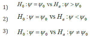
directly from the significance function.
Let us first consider p(ψ) is an increasing function of ψ. Then
i.  satisfies
  and
and 
ii. p-values for testing the corresponding hypotheses are

However, if p(ψ) is a decreasing function of ψ, then
a) 
b) p-values for testing the corresponding hypotheses are

To continue with our blood phosphorus level example from the previous section, the confidence interval is recorded in Figure 1. Since p(μ) is a decreasing function of ,μ and we are testing the hypothesis H0:μ>4.8 vs Ha:μ=4.8 hence, the p-value is 1-0.954=0.046. Note that one-sided confidence intervals and confidence intervals with minimum width can also be obtained from the significance function.
Applications of the significance function
In this section, we use two examples to illustrate the application of the significance function.
Example 1: Grice & Bain [7] reported the survival times of male mice exposed to gamma radiation in weeks. The data are:

An exponential model is used to analyze this dataset. More specifically, let iT be the survival time of the thi mice exposed to gamma radiation. Then,
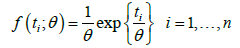
Where t0=2269 is the observed total survival times, and g(t;θ) is the probability density function of the gamma distribution with shape n and scale .θ Figure 2 gives the significance function and we can see that the 95% confidence interval for the mean survival time is (76.57, 187.73) weeks. To test the hypothesis H0:θ>80 vs Ha:θ≠80 from Figure 2, we have p(80)=0.9583. Since p(θ) is a decreasing function of θ and we have a two-sided test, the corresponding p-value is 2(1-0.9583)=0.0834. Thus, 8.34% of potential data values are at least as extreme as the observed data, relative to the distribution with the parameter 80.θ=


Example 2: Kieler et al. [8] reported that the pregnancy length in singleton pregnancies with a spontaneous onset labour, calculated from bipariental diameter of 509 mothers who are smokers, had a mean of 280.3 days and a standard deviation 8.2 days. Assume the length of these types of pregnancy is normally distributed. The parameter of interest is the precision parameter ,ψ which is the reciprocal of the variance parameter. Since, (n-1)S2ψ− is distributed as a Chi-square distribution with (n-1) degrees of freedom, where 2S is the observed sample variance. Then the significance function is  which is given in Figure 3. As indicated in Figure 3, a 90% confidence interval for ψ is (0.0134,0.0164). In testing the hypothesis H0:ψ>80 vs Ha:ψ≠80 we have ()0.0150.5626.p= Since p(ψ) is an increasing function ,ψ and we have a two-sided test, the corresponding p-value is 2(1-0.5625)=0.8748..Thus, 87.48% of potential data values are at least as extreme as the observed data, relative to the distribution with the parameter 0.015.
Conclusion
In this paper, we defined the significance function and demonstrated how it can be applied. Our illustrative examples showed that we can obtain both confidence intervals and p-values with ease directly from the significance function. Throughout this paper, we assumed that the significance function exists explicitly. However, in practice, this may not be the case. In these situations, there are standard approximations that can be used, such as the likelihood based methods (Wald method, Rao method, and the Wilks method), to obtain an approximate significance function. Applications of the likelihood based methods can be found in many books, such as Lawless [9], Kalflesich & Prentice [10], and Brazzele et al. [11].
References
- Neyman J (1937) Outline of a theory of statistical estimation based on the classical theory of probability. Phil Trans Roy Soc A 236: 333-380.
- Moore DS, McCabe GP, Craig BA (2014) Introduction to the practice of statistics (8th edition) W.H. Freeman and Company: New York, USA.
- Susic JM (1985) Dietary phosphorus intakes, urinary and peritoneal phosphate excretion and clearance in continuous ambulatory dialysis patients. MS thesis, Purdue University.
- Fraser DAS (2017) p-Values: The insight to modern statistical inference. Annu RevStat Appl 4: 1-14.
- Fisher R (1956) Statistical methods and scientific inference. Oliver and Boyd: London, UK.
- Fraser DAS (2018) p-Values: What are they? Who do we ask? Biostat Biom Open Access J 6: BBOAJ.MS.ID.555693.
- Grice JV, Bain LJ (1980) Inferences concerning the mean of the gamma distribution. J Am Stat Assoc 75: 929-933.
- Kieler H, Axelsson O, Nilsson S, Waldenstro U (1995) The length of human pregnancy as calculated by ultrasonographic measurement of the fetal biparietal diameter. Ultrasound Obstet Gyencol 6: 353-357.
- Lawless JF (2003) Statistical models and methods for lifetime data (2nd Edn). John Wiley & Sons, Inc: New Jersey, USA.
- Kalbeisch JD, Prentice RL (2002) The statistical analysis of failure time data (2nd Edn). John Wiley & Sons, Inc: New Jersey, USA
- Brazzale AR, Davison AC, Reid N (2007) Applied asymptotics: Case studies in small-sample statistics. Cambridge University Press: Cambridge, UK.


