


AHybrid Solutions Method for Solving One Dimensional Parabolic Partial Differential Equations
Sunday Babuba*
Department of Mathematics, Federal University Dutse, Nigeria
Submission: March 19, 2018; Published: July 02, 2018
*Corresponding author: Sunday Babuba, Department of Mathematics, Federal University Dutse, Nigeria, Tel: ; Email: vishaaldeo@gmail.com
How to cite this article: Sunday B. AHybrid Solutions Method for Solving One Dimensional Parabolic Partial Differential Equations. Biostat Biometrics Open Acc J. 2018; 7(3): 555713. DOI: 10.19080/BBOAJ.2018.07.555713
Abstract
A new continuous numerical method based on polynomials approximation is here proposed for solving the equation arising from heat transfer along a copper rod and a hollow tube subject to initial and boundary conditions. The method results from discretization of the heat equation which leads to the production of a system of algebraic equations. By solving the system of algebraic equations we obtain the problem approximate solutions.
Keywords: Polynomials; Interpolation; Multistep collocation; Parabolic partial differential Equations; Numerical method; One dimensional; Hybrid solutions; Algebraic equations; Heat equation; Heat conduction equation; Interpolation; Collocation; Temperature; Heat flow; Polynomials; Numerical accuracy; Evaporates; Zero; Ethyl alcohol; Initial temperature; Interpolation point.
Introduction
The development of continuous numerical techniques for solving heat conduction equation in science and engineering subject to initial and boundary conditions is a subject of considerable interest. In this paper, we develop a new numerical method which is based on interpolation and collocation at some point along the coordinates [1-3]. To do this we let U(x,t) represents the temperature at any point in the rod and the tube. Heat is flowing from one end to another under the influence of temperature gradient .Ux∂∂ To make a balance of the rate of heat flow in and out of the media, we consider R for thermal conductivity of the steel, C the heat capacity which we assume constants, and ρ the density and D the thermal diffusivity of alcohol. Heat flow in the rod is given by

Where A and B are the cross sections of the rod and the tube respectively. Our new method strives to provide solutions to the heat flow eqns. (1.0) and (1.1).
The solution method
To set up the solution method we select an integer N such that .0>N We subdivide the interval Xx≤≤0 into N equal subintervals with mesh points along the space axis given by 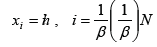 , where .Nh=X Similarly, we reverse the roles
of x nd t, we select another integer Msuch that .0>M We also subdivide the interval Tt≤≤0 into M equal subintervals with mesh points along time coordinate given by
, where .Nh=X Similarly, we reverse the roles
of x nd t, we select another integer Msuch that .0>M We also subdivide the interval Tt≤≤0 into M equal subintervals with mesh points along time coordinate given by 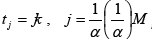 , where ,TMk= and kh, are the mesh sizes along space and time coordinates [4-6]. We seek for the approximate solution
  , to U(x,t), of the form

over h>0,k>0 mesh sizes, such that  . We denote p to be the sum of interpolation points along the space and time coordinates respectively. That is ,bgp+= where g is the number of interpolation points along the space axis, while b is the number of interpolation points along the time coordinate [7]. The bases functions rrsqr,sr1,...p-1rare the Taylor’s and Legendre’s polynomials which are known, raare the constants to be determined. The interpolation values
 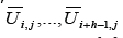 are assumed to have been determined from previous steps, while the method seeks to obtain
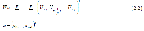
Applying the above interpolation conditions on eqn. (2.0) we obtain

We let 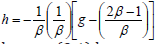 arbitrarily and k=0, then by Cramer’s rule, eqn. (2.1) becomes
and 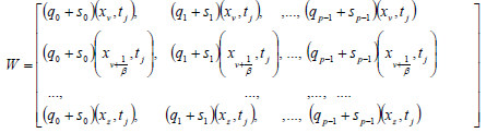
Where 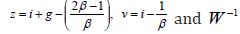 exist. Hence, from eqn. (2.2), we obtain

The vector  is now determined in terms of known parameters in
  , then
Substituting eqn. (2.4) into eqn. (2.5) we obtain
We reverse the roles of x and t in eqn. (2.1) and we arbitrarily set 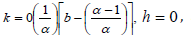 again by Cramer’s rule, eqn. (2.1) become
and 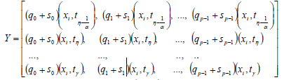
where 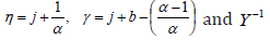 exist.
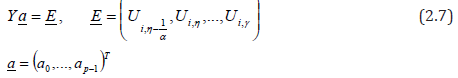
Hence, from eqn. (2.7) we obtain

The vector is now determined in terms of known parameters in  row of ,L then

Also, eqn. (2.9) determines the values of ar explicitly.
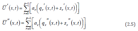
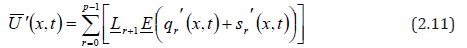
Taking the first derivatives of eqn. (2.0) with respect to t we obtain
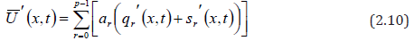
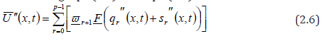
Substituting eqn. (2.9) into eqn. (2.10) we obtain
But by eqns. (1.0) and (1.1) it is obvious that eqn. (2.11) is equal to eqn. (2.6), therefore,
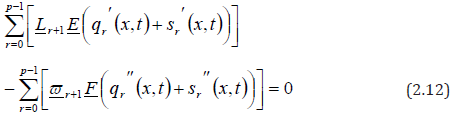
Collocating eqn. (2.12) at ixx= and jtt= produces a new numerical scheme that solves equations (1.0) and (1.1) explicitly.
Numerical examples
In this section, we will test the numerical accuracy of the new method by using the new scheme to solve two examples. That is, we compute an approximate solutions of eqns. (1.0) and (1.1) at each time level. To achieve this, we truncate the polynomials after second degree and the average is used as the basis function in the computation [8-10]. The resultant scheme is used to solve the following problems.
Example 1
A hollow tube 20 cm long is initially filled with air containing 2% of ethyl alcohol vapors [2]. At the bottom of the tube is a pool of alcohol which evaporates into the stagnant gas above. (Heat transfers to the alcohol from the surroundings to maintain a constant temperature of 30 °C, at which temperature the vapour pressure is 0.1 atm.) At the upper end of the tube, the alcohol vapors dissipate to the outside air, so the concentration is essentially zero. Considering only the effects of molecular diffusion, determine the concentration of alcohol as a function of time and the distance x measured from the top of the tube.
Molecular diffusion follows the law
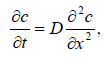
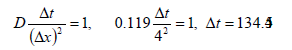
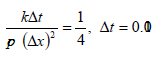
Where, D is the diffusion coefficient, with units of cm2/sec. (This is the same as for the ratio k/cp, which is often termed thermal diffusivity.) For ethyl alcohol, D = 0.119 cm2/sec at 30 °C , and the vapor pressure is such that 10 volume percent alcohol in air is present at the surface [11-15]. The initial condition is ()0.20,=xc, and boundary conditions are ()()10,20,0,0==tctc. Subdivide the length of the tube into five intervals, so that xΔ = 4cm. Using the maximum value permitted for tΔ yields
Taking 32,4==αβ implies that 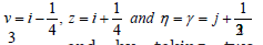 For
For 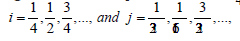 and by taking two interpolation points along space coordinate and one interpolation point along time coordinate implies that 3,1,2=⇒==pbg, and this simply means that
 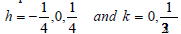 then the calculated concentration of alcohol is as shown in Table 1 [15-20].

Example 2
Solve for the temperature in a copper rod 1.2 cm long, with the outer curved surface insulated so that heat flows in on one direction [21-24]. If the initial temperature ()Co within the rod are given by

Find the temperature as a function of x and t if both faces are maintained at 0° C. For copper, 433.0,37.0==cpk. We use ,20.0cmx=Δ we then find tΔ by the relation
Taking 32,4==αβ implies that 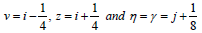 .For
.For 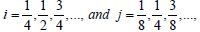 and by taking two interpolation points along space coordinate and one interpolation point along time coordinate implies that ,1,2==bgand 3=p, this simply gives 81,041,0,41=−=kandh, then the calculated temperatures are as shown in Table 2 [25-27].

References
- Adam A, David R (2002) One dimensional heat equation.
- Awoyemi DO (2002) An Algorithmic collocation approach for direct solution of special fourth- order initial value problems of ordinary differential equations. Journal of the Nigerian Association of Mathematical Physics 6: 271-284.
- Awoyemi DO (2003) A P– stable linear multistep method for solving general third order Ordinary differential equations. Int J Computer Math 80(8): 987-993
- Bao W, Jaksch P, Markowich PA (2003) Numerical solution of the Gross-Pitaevskii equation for Bose-Einstein condensation. J Compt Phys 187(1): 18-342
- Benner P, Mena H (2004) BDF methods for large scale differential Riccati equations in proc. of mathematical theory of network and systems. MTNS.
- Bensoussan A, Da Prato G, Delfour M, Mitter S (2007) Representation and control of infinite dimensional systems, (2nd edition), Springer, UK
- Biazar J, Ebrahimi H (2005) An approximation to the solution of hyperbolic equation By a domain decomposition method and comparison with characteristics Methods. Appl Math and Comput 163(2): 633-648.
- Brown PLT (1979) A transient heat conduction problem. AICHE Journal 16: 207-215.
- Chawla MM, Katti CP (1979) Finite difference methods for two-point boundary value problems involving high–order differential equations. BIT 19(1): 27-39.
- Cook RD (1974) Concepts and Application of Finite Element Analysis: NY: Wiley Eastern Limited, USA
- Crandall SH (1955) An optimum implicit recurrence formula for the heat conduction equation. JACM 13: 318-327
- Crane RL, Klopfenstein RW (1965) A predictor-corrector algorithm with increased range of absolute stability. JACM 12: 227-237.
- Crank J, Nicolson P (1947) A practical method for numerical evaluation of solutions of partial differential equations of heat conduction type. Proc Camb Phil Soc 6: 32-50.
- Dahlquist G, Bjorck A (1974) Numerical methods. NY: Prentice Hall
- Dehghan M (2003) Numerical solution of a parabolic equation with non-local boundary specification. Appl Math Comput 145(1): 185-194.
- Dieci L (1992) Numerical analysis. SIAM Journal 29(3): 781-815
- Douglas J (1961) A Survey of Numerical Methods for Parabolic Differential Equations in advances in computer II. Academic press, USA.
- D’ Yakonov, Ye G (1963) On the application of disintegrating difference operators. Z Vycist Mat I Mat Fiz 3: 385-395.
- Eyaya BE (2010) Computation of the matrix exponential with application to linear parabolic PDEs.
- Fox L (1962) Numerical Solution of Ordinary and Partial Differential Equation. New York: Pergamon, USA.
- Penzl T (2000) Matrix analysis. SIAM J 21: 1401-1418.
- Pierre J (2008) Numerical solution of the dirichlet problem for elliptic parabolic Equations. SIAM J Soc Indust Appl Math 6(3): 458-466.
- Richard LB, Albert C (1981) Numerical analysis. Berlin: Prindle, Weber and Schmidt, inc, USA.
- Richard L, Burden J, Douglas F (2001) Numerical analysis, (7th edn), Berlin: Thomson Learning Academic Resource Center, USA.
- Saumaya B, Neela N, Amiya YY (2012) Semi discrete Galerkin method for Equations of Motion arising in Kelvin-Voitght model of viscoelastic fluid flow. Journal of Pure and Applied Science 3(2&3): 321- 343.
- Yildiz B, Subasi M (2001) On the optimal control problem for linear Schrodinger equation. Appl Math and Comput121: 373-381
- Zheyin HR, Qiang X (2012) An approximation of incompressible miscible displacement in porous media by mixed finite elements and symmetric finite volume element method of characteristics. Applied Mathematics and Computation, 143: 654 - 672.


