Research Article

Complexities on Median Calculation

M A Jalil and Jamil H Karami*

Department of Statistics, University of Dhaka, Bangladesh

Submission: February 08, 2018; Published: May 05, 2018

*Corresponding author: M A Jalil, Department of Statistics, University of Dhaka, Dhaka-1000; Bangladesh, Tel: (+88)01974799788; Fax: 880-2-9667222; email: majalil@du.ac.bd

How to cite this article: M A Jalil, Jamil H K. Complexities on Median Calculation. Biostat Biometrics Open Acc J. 2018; 7(1): 555705. DOI: 10.19080/BBOAJ.2018.07.555705

Abstract

The complexity of median calculation is explored with some examples in this article. We have pointed out how to identify ungrouped and grouped data, and thereby the appropriate method of computing median and other percentiles.

Keywords: Ungrouped data; Grouped data; Median; Percentile; Location parameter; Ungrouped; Frequency; Evaluating median; Sample data; Values; Distribution; Continuous scale; Repeated values; Domain; Horizontal line; Equal halves; Lower boundary; Cumulative frequency; Statistical packages; Economic status; Central tendency

Introduction

Location is an important measure in describing a sample data for a variable. For a discrete or ordinal data we can calculate percentiles for location parameter. Among these location parameters, the median is the most important one in describing a variable, as it informs the central position of the distribution underlying variable. In this article, we show the importance of identifying whether a data set is ungrouped or grouped. Although some articles have questioned about the usefulness of grouped data [1], we think the existence of grouped (frequency) data is very frequent in real-world examples compared to ungrouped data. In this research, we have suggested an appropriate method of computing median and other percentiles. The concept has been illustrated with several examples.

Methods

Several methods can be used for evaluating median from sample data [2]. It is crucial to decide which of them would be appropriate for the problem at hand. This difficulty can be resolved if we simply think of the nature of the data for a particular problem. By the `nature’ we mean whether a data set is grouped or ungrouped. If we have raw data (observed) of a continuous variable with no repeated observations (i.e., single frequency for each case), the data is called ungrouped data. Suppose, three values of grades obtained by a student are 2.8, 2.9 and 3.3; it is an example of ungrouped data. Therefore, we can compute median using the formula for ungrouped data. However, in real world examples, the ungrouped data is not frequently encountered. It is hardly possible to get scope of work with this type of data. On the other hand, if there are any repeated observations in the data set, it is called a grouped data. If the three values of grades were 2.8, 2.8 and 3.3, it can be considered as grouped data. In fact, practically observed data obtained from any field of enquiry or experiment for a continuous variable is mostly grouped data, frequency of one or more observations are present.

Median is the middlemost location of a distribution or of a set of values for a variable with respect to number of observations. To find the median, we locate the center point keeping 50% observations left to the point and 50% observations to the right of a distribution. The value corresponding to this center point is the median. Percentiles are measures of location and median is the 50th percentile. Median lies on a continuous scale corresponding the domain of the variable under consideration. It is interesting to note that whatever be the type of a variable, median is always continuous. For an observed set of values we can scale a horizontal line with the values and locate the point where it divides into two equal halves with respect to number of observations. The value on the scale of the located point is the median.

Results and Discussion

For an ungrouped raw data the median is calculated as: x₁,x₂,....,x_n (ordered). If number of observations (n) is odd, the sample median is the n + 1^th/2 observation. But if there are repeated values in the central area of the distribution (of underlying variable), then n + 1^th/2 observation may not be the median. We illustrate this with an example [3].

Example 1

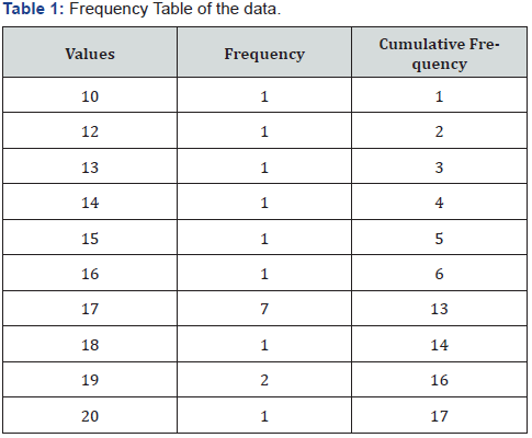
Let us consider some observations: 10, 12, 13, 14, 15, 16, 17, 17, 17, 17, 17, 17, 17, 18, 19, 19, 20. Clearly, n +1/2=17+1/2=9^th observation = 17, which many people will take as median. But, if we notice carefully it can be seen that 7^th, 8^th, 10^th, 11^th, 12^th and 13^th observations are also 17. Therefore, the value actually does not divide the whole distribution into two equal halves. Still then, how can we accept it as median?

We have mentioned in the methods section that this data set is actually a grouped data. It would be appropriate to use the formula prescribed for the grouped data. Remember the formula for computing th percentile:

where, L_k is lower boundary of median class, k F_−k is cumulative frequency of pre k^th percentile class, f_k is frequency of k^th percentile class, and C_w is k^th percentile class width. Here, L_k is used for a grouped data. The data in this example is represented in Table 1. From this table, the median class is to be considered 16.5 −17.5.

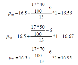
Using the formula mentioned above, we have p₅₀ =16.7. However, for this same problem, p₅₀ will be determined as 17 in many books and statistical packages as discussed earlier. The reason behind this is that they consider this type of data set as ungrouped data, which is not appropriate according to our definition of grouped and ungrouped data. It is interesting to note that if someone considers the data as ungrouped, then p₄₀ , p₄₁ ,...., p₇₅ are all equal. That is, in this case, all percentiles from 40^th to 75^th are equal to 17. This contradicts the concept of percentile. On the other hand, if we consider the data set as grouped data (frequency data), we have the following percentiles:

It is remarkable that the above percentile calculations seem rather appropriate.

Example 2

Suppose we have the following data on economic status (1: high class, 2: high-middle class, 3: middle class, 4: lower-middle class and 5: lower class):

1, 1, 1, 2, 2, 2, 2, 2, 3, 3, 3, 3, 3, 3, 3, 3, 4, 4, 5.

We show how the suggested method can be used to describe the economic status with the measures of central tendency and dispersion. Using the method, it is easy to find that the central tendency (median) is 2.51, and dispersion (quartile deviation) is 0.72.

Example 3

Suppose we are given test scores of 100 students as in Table 2. This type of examples are available in Ross [4]. Using the suggested method, we have found the following percentiles: Median = 50^th percentile = 5.625; 60^th percentile = 5.875; 70^th percentile = 6.125; 80^th percentile = 6.375. However, if these percentile were calculated otherwise (i.e., considering this data set as ungrouped), then 50^th to 80^th percentiles will all be equal to 6, which is not acceptable at all.

Conclusion

It is very rare to find an ‘ungrouped data’ where each of the values will occur only once. We can assume an ungrouped data theoretically, but practically it is rare. In contrary, grouped data is very common. We recommend the formula for grouped data in the calculation of median and other percentiles. The formula for grouped data is appropriate with all of the examples we mentioned here and beyond.

Acknowledgement

This research has been supported by Dhaka University research allowance.

References

1. Freund EJ, Perles MB (1987) A new Look at Quartiles of Ungrouped Data. The American Statistician 41(3): 200-203.
2. Hyndman JR, Fan Y (1996) Sample Quantiles in statistical Packages. The American Statistician 50(4): 361-365.
3. Downie NM, Heath RW (1970) Basic Statistical Methods. Harper International, USA.
4. Ross MS (2010) Introductory Statistics (3rd edn). Academic Press, USA