


An Investigation of the Discriminatory Ability of the Clustering Effect of the Frailty Survival Model
Robin Van Oirbeek* and Emmanuel Lesaffre
Department of Biostatistics and Statistical Bioinformatics, KU Leuven University, Belgium
Submission: November 01, 2017; Published: April 25, 2018
*Corresponding author: Robin Van Oirbeek, Department of Biostatistics and Statistical Bioinformatics, Katholieke Universiteit Leuven and Universiteit Hasselt, Belgium, Tel: 0032 485 920629; Email: robin.vanoirbeek@gmail.comHow to cite this article: Robin Van O, Emmanuel L. An Investigation of the Discriminatory Ability of the Clustering Effect of the Frailty Survival Model. Biostat Biometrics Open Acc J. 2018; 6(3): 555688.DOI:10.19080/BBOAJ.2018.06.555688
Abstract
A strategy is proposed to examine the importance of the clustering effect of the frailty model by means of the concordance probability. To this end, the methodology proposed in earlier work is extended to general frailty models and a new definition of the concordance probability is developed. The resulting measures allow to separate the discriminatory ability of the covariate effects and the clustering effect on a within- and between-cluster level. Using a Bayesian and a likelihood approach, point estimates and 95% credible/ confidence intervals are computed for the measures. Estimation properties and sensitivity against misspecification are checked in an extensive simulation study. As such, the likelihood estimation procedure showed difficulties in estimating unbiasedly the predictive ability of the clustering effect, while the Bayesian estimation procedure resulted in good estimation properties for all three measures. Other features are developed to complement the earlier methodology, such as an internal validation strategy as well as a procedure to calculate internally validated interval estimates in the presence of clustered data. The ensemble of the developments is illustrated on a dental data set.
Keywords: Clustered data; Concordance probability; Discrimination; Frailty model; Predictive ability
Abbreviations: IPCW: Inverse Probability Censoring Weighted; MSE: Measures The Empirical; PH: Proportional Hazards
Introduction
The frailty model is a popular model to analyze clustered survival data. For this model, the importance of clustering typically is assessed by means of the variance of the frailty distribution only: when the variance is large, clustering is important and visa versa. In this article we would like to investigate the importance of clustering in more detail. To this end, we propose to assess how clustering affects the quality of the model predictions. Despite the importance of the frailty model, few predictive measures have been suggested for the frailty model. To our knowledge, only the concordance probability has been extended to PH frailty models, resulting in 3 separate versions of the concordance probability [1]. These 3 concordance measures allow to evaluate the discriminatory ability on a within-cluster and between-cluster level separately and to measure the predictive gain of the clustering effect on top of the covariate effects. The methodology in [1] shows, however, two major shortcomings which will be tackled in this article.
The first shortcoming in [1] is that the concordance probability is estimated using Harrell's C estimation technique. The disadvantage of this estimation technique is that, in the presence of censoring, it suffers from a bias that depends on the censoring distribution. Moreover, this estimation technique is only designed for a time-unrestricted definition of the concordance probability that assumes survival models with non-crossing survival curves. In this article, we make use of a Inverse Probability Censoring Weighted (IPCW) estimator of[2] designed for the time-restricted definition concordance probability of [3]. This IPCW estimator is proven to be consistent, given that the censoring model is correctly specified. The time-restricted definition of the concordance probability has the advantage that it can be applied to any survival model. Moreover, we also introduce a new time restricted definition of the concordance probability, bearing a slightly different interpretation than the one introduced by [3]. Note that this shortcoming has also been addressed by [4], but their IPCW estimator assumes the PH frailty model as the survival model and a censoring distribution that does not depend on covariates. The second shortcoming in [1] is that their methodology is insufficiently tailored to its use in practice. As such, we provide an internal validation procedure to correct the estimated concordance probabilities for over optimism when the data set is used for both model fitting and model evaluation. For this, we adapt the internal validation procedure proposed for the Brier score for univariate survival data [5]. We also show how one can calculate an interval estimate for the overoptimistic and the internally validated concordance probability of interest.
In Section 2.1, the time-unrestricted, the time-restricted definition of [3] and the new time-restricted definition of the concordance probability are introduced for univariate survival data. In Section 2.2, it is shown how these definitions can be adapted for frailty model in general, including interval estimates. The estimation of internally validated point estimates is dealt with in Section 2.3. The estimation properties of the two time-restricted definitions of the concordance probability using a Bayesian and a likelihood approach are investigated in Section 3.1 by means of a large-scale simulation study. The effect of misspecifying the frailty distribution and the censoring model on the estimation of the concordance measures is shown in Section 3.2. All developments are applied to a dental data set in Section 3.3, followed by a discussion in Section 4.
Methods
Different concordance probabilities
In Section 2.1, the time-unrestricted, the time-restricted definition of [3] and the new time-restricted definition of the concordance probability are introduced for univariate survival data. In Section 2.2, it is shown how these definitions can be adapted for frailty model in general, including interval estimates. The estimation of internally validated pIn the next section, one time-unrestricted and two time- restricted definitions of the concordance probability are shown for univariate survival data, after which for each respective definition its common estimation technique is discussed.
Definitions
In Section 2.1, the time-unrestricted, the time-restricted definition of [3] and the new time-restricted definition of the concordance probability are introduced for univariate survival data. In Section 2.2, it is shown how these definitions can be adapted for frailty model in general, including interval estimates. The estimation of internally validated p[6] proposed the unrestricted concordance probability C which is the earliest definition of the concordance probability. It equals the probability that a randomly selected subject i, which fails later than another randomly selected subject j, has a higher predicted survival time than subject j or,
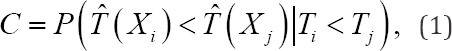
With  the true failure time, the time- independent predicted failure time (e.g. median survival time) and the covariate vector of the failure time model of subject i. Since the subjects of a survival study are followed up over a limited time period, the estimation of the concordance probability should be regarded as particular to the study. The above definition, however, gives the impression that it applies to the whole time range, since no time restriction is imposed on the pairs of subjects that are evaluated in the above definition. As a result, the use of (1) in a study with a limited follow-up implies that the same survival process holds beyond the last follow-up time, which is an unverifiable assumption. Moreover, since (1) evaluates the ranking of the time-independent predicted failure times
  of a pair (i, j), the survival probability at time point
  can only be used as a predictor when its ranking is not time dependent, which does not hold for all failure time models. A restricted version of the concordance probability CT was therefore introduced by [3], i.e.:

With  representing the time-dependent predicted failure time (e.g. survival probability at a certain time point ).
Measures how well subjects, who fail before time point τ can be distinguished from subjects that fail later than the considered subject. Different τ values can be chosen to investigate how earlier failing subjects are differentiated from later failing subjects over time. In practice however, it might also be of interest to examine how well subjects are discriminated when their true failure times are close to each other as compared to when their true failure times differ greatly. To investigate this, we propose a new concordance measure:
representing the time-dependent predicted failure time (e.g. survival probability at a certain time point ).
Measures how well subjects, who fail before time point τ can be distinguished from subjects that fail later than the considered subject. Different τ values can be chosen to investigate how earlier failing subjects are differentiated from later failing subjects over time. In practice however, it might also be of interest to examine how well subjects are discriminated when their true failure times are close to each other as compared to when their true failure times differ greatly. To investigate this, we propose a new concordance measure:

With d the maximum difference in true failure time between the two randomly selected subjects. As such, (3) measures how well subjects with a maximum difference d in failure time can be distinguished from each other, given that the earliest failing member of the pair fails before time pointτ Plotting CT(d) versus different values of d provides a more detailed image of the discriminatory ability of the failure time model. Note that we propose to use the survival probability at time point 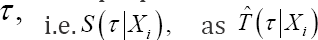 for definitions (2) and (3) since it captures the cumulative risk for the event in [0,τ].
Estimation
For a sample of size n, consider a subject i(i = 1----n) with observed failure timeti = min(Ti,Ci) andci its censoring time. The censoring indicatorδiequals 1 if ti = Ti and 0 otherwise. The unrestricted concordance probability C is typically estimated by Harrell's estimation technique [6] or:
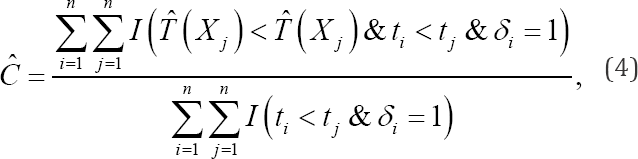
With Xi the observed covariates of the failure time model of subject i. Pairs that agree with the condition in the denominator (numerator) of the upper formula are called comparable (concordant) pairs. As proven by [2], (4) is known to suffer from an overoptimistic bias that depends on the censoring distribution. In the remainder of this article, we will no longer consider this estimation technique of the concordance probability. [2] proposed the Inverse Probability Censoring Weighted (IPCW) estimation method for the CT definition, which corresponds to:
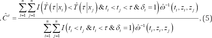
with 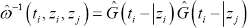 the estimated censoring weight of the pair (i, j),ti- the time point just before ti and G (t\zi) the survival probability of the censoring model and Zi the observed covariates of the censoring model of subject at time point t Clearly, lim
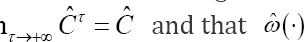 s equal to 1 when all subjects are uncensored.
Just as for Harrell's estimation technique of C, (5) only considers concordant pairs in the numerator and comparable pairs in the denominator, but each pair is multiplied with its estimated corresponding censoring weight The censoring weights are obtained by means of a censoring model, which is fitted to the data by reversing the meaning of the censoring indicator: the true censoring time is censored when the event occurred (δ=1), and uncensored when the event did not occur (δ = 0). Further, (5) estimates CT consistently under conditional independence of the censoring mechanism and the failure time model and if the censoring model is correctly specified. Hence, because the censoring weights only depend on the censoring model, estimator (5) is robust against misspecification of the failure time model [2]. The censoring weights therefore compensate for the use of just comparable pairs in the estimation of CT, counterbalancing the overoptimistic bias that would have been obtained else wise. Note that the covariates X and Z of the failure time model and the censoring model respectively are not necessarily the same.
Following [2], we have developed the following consistent IPCW estimator of Cτ( d):
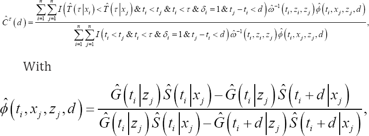
The additional weight of the pair (i,j). Clearly,  and lim
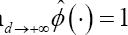 such that iim
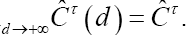 Moreover,
  and are both equal to 1 when all subjects are uncensored. In (6), is needed because
  requires a quantification of the probability that the difference in failure time of the considered pair is lower than d in the presence of censoring. Further, since depends on both the failure time model and the censoring model, (6) is a consistent estimator of CT (d) only when both models are correctly specified. The derivation of (6) as well as the proof of its consistency are shown in Appendix.
Application to the frailty model
The concordance probability has already been adapted to the framework of Proportional Hazards (PH) frailty models of the power variance family for the unrestricted definition (1) of the concordance probability [1]. In this section, we will extend the concordance probability to the whole class of frailty models. In the next two sections, we restrict ourselves to definition (2). For the developments related to definition (3), we refer to Section A of the online supplementary material.
Definition
The frailty model is a popular model for clustered survival data. For each subject of cluster q a frailty term wq is introduced to account for clustering. These frailty terms are assumed to be sampled from a frailty distribution, fw (w) ? which mostly is a parametric distribution such as the gamma distribution [7]. For each frailty model two different types of survival probabilities can be defined for a given time poin τ,i.e. a conditional survival probability  and a marginal survival probability
  [7]. Note that
  takes covariate and cluster information into account, while
  just accounts for covariate information. For the PH frailty model for instance, it holds that
 the cumulative
baseline hazard at time point τ and β a vector of regression coefficients. For PH frailty models of the power variance family
the cumulative
baseline hazard at time point τ and β a vector of regression coefficients. For PH frailty models of the power variance family
 with Clearly
 depends on the choice of the frailty
distribution, while
depends on the choice of the frailty
distribution, while  does not.
Two types of pairs can be identified for clustered data: an inter-cluster pair, whose members belong to two different clusters, and an intra-cluster pair, whose members belong to the same cluster. Therefore, depending on which type of pair and survival probability is used, 6 different versions of the concordance probability can be introduced for frailty models (Table 1). This results in a between marginal and a between conditional concordance probability CTBM and CTBC, respectively, in a within marginal and a within conditional concordance probability CTWM and CTWC, respectively, and in an overall marginal and an overall conditional concordance probability CTOM and CTOC respectively.

Interpretation and interrelations
For the two overall concordance probabilities, it can be shown that  with
with  the probability that a pair is an inter-(intra-)cluster pair [1]. As a result,CTOC and CTOM do not add new information to the other 4 versions of the concordance probability. Moreover, their interpretation depends strongly on the sampling scheme of the data structure such that its value is hard to compare across studies with different clustering designs [1]. Since the properties of CTOC (CTOM ) depend on the properties of CTBC and CTWC (CTBC and CTWM) we will not consider the overall measures CTOC and CTOMany further. For PH frailty models of the power variance family, it has been shown that CTWC= CTWM = CTW holds [1]. In Appendix B, we proof the latter result holds for each frailty model. This means that we can either use the conditional or the marginal survival probabilities in the calculation of CTW In addition, when the failure time model is correctly specified, it can be shown thatCTBC ≥ CTBM for all frailty models [1].
Summing up, only 3 unique versions of the concordance probability can be defined for the frailty model and each of these definition focuses on a specific aspect of the frailty model. CTBC measures the inter-cluster predictive ability of the covariate effects and the clustering effect, while CTBM measures the intercluster predictive ability of the covariate effects only. Comparing CTBC and CTBM indicates how much CTBMwould increase if the clustering effect were completely captured by the covariate effects. CTW measures the intra-cluster predictive ability of the cluster varying covariate effects.
Computation of point estimates
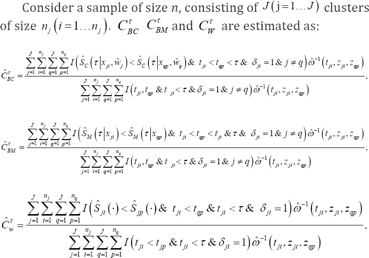
With tji,xji,zjiSji the observed failure time, the covariate vector of the failure time model and the censoring model and the censoring indicator for subject of cluster  equals either
Following the definition of CTBM and (7), the marginal survival probability needs to be calculated for each subject at time point τ in the estimation of CTBM This survival probability is, however, hard to compute for most frailty models due to the integration step. Also, the marginal survival probability depends on the choice of the frailty distribution, while the conditional survival probability does not. In Appendix B, we prove that the ranking of  in the calculation of CTBM is the same as the ranking of <
 treating the considered pair (incorrectly) as an intra-cluster pair. As a result, the evaluation of CTBMcan also be completed by means of the conditional survival curves only. Since CTW can be obtained by determining the ranking of the conditional survival curves only, the same ranking rule for the predicted failure times can be established for CTBM and CTW for a class of frailty models, applying this ranking rule to inter-cluster pairs for CTBM and to intra-cluster pairs for CTW As such, only the ranking of the linear predictors is needed in the estimation CTBM of CTBM and of the PH frailty model, since:

In summary, a ranking rule for the predicted failure times needs to be established for CTBC using assuming that both members of the pair belong to a different cluster and for CTBM and CTW using
  assuming that both members of the pair belong to the same cluster.
Computation of interval estimates
A credible/confidence interval is constructed by means of a Bayesian/likelihood procedure, combined with the percentile non-parametric bootstrap of [8]. This bootstrapping technique has been adapted to the clustered data setting, i.e. resampling by cluster and always selecting the same number of clusters in each bootstrap sample [9]. When the failure time model is fitted using likelihood or a Bayesian approach, the censoring model needs to be fitted using the same approach. Even if credible intervals can be readily obtained for the Bayesian procedure from the posterior distribution of the respective concordance probabilities, the bootstrap technique is necessary to ensure that the resulting 95% credible interval captures the uncertainty of the estimation of the model parameters for future values of the observed covariates [1]. The description of both procedures using the BCα method [8], which is a more refined version of the percentile non-parametric bootstrap method, can be found in Section B of the online supplementary material. Since the developments for the three measures are the same, we denote the measure of interest as CT. The Bayesian procedure then corresponds to:
a. After removing the burn-in part of the Markov chain, let the MCMC procedure run for an extra m iterations. At iteration p with p = 1,...,m of the MCMC sampling process determine the posterior estimate for each model parameter. For the PH frailty model, posterior estimates for the parameters of the baseline hazard function ^0 (t), the covariate effects β and the frailty terms w are obtained in this manner [7]. This step needs to be applied to the failure time model and the censoring model separately.
b. For each subject obtain the posterior sample of the censoring weight based on the posterior sample of the censoring model parameters.
c. Compute CT(l) at each iteration l withl = I----,m based on the posterior sample of the failure time model parameters and the posterior sample of the censoring weightsω(.). We suggest to take the median of the posterior values of CT(l) is the point estimate Ct.
d. Apply the Bayesian bootstrap technique of [10] to sample k = 1,...,k new bootstrapping data sets. Calculate the point estimate of each kth bootstrap data setĈT(K) based on the posterior samples ĈT(l,K)
e. Compute the 95% credible interval (CI) by means of the percentile method of [8] using the point estimates of the K bootstrap data sets ĈT(K) As such, the 2.5 and the 97.5 percentile of the bootstrap point estimates ĈT(K) constitute the lower and the upper bound of the 95% credible interval ĈT of
The likelihood procedure is equal to:
a) Determine the point estimates of the model parameters, which are obtained for the PH frailty model by maximizing the marginal likelihood for the parameters of the baseline hazard function ^o (t) and the covariate effects β after which empirical Bayes estimates are calculated for the frailty terms [7]. This step needs to be applied to the failure time model and the censoring model separately.
b) For each subject obtain the point estimate of censoring weightωi(.) based on the estimates of the censoring model parameters.
c) Compute the point estimate ĈT based on the estimates of the failure time model parameters and point estimates of the censoring weights ω(.).
d) Apply the bootstrap technique of [8] to sample k = 1,..., k new bootstrap data sets. Calculate the point estimates of eachkth bootstrap data set ĈTk).
e) Compute the 95% confidence interval (CI) by means of the percentile method of [8] using the point estimates of the K bootstrap data sets ĈTk) As such, the 2.5 and the 97.5 percentile of the bootstrap point estimates ĈTk) constitute the lower and the upper bound of the 95% confidence interval of Ct.
Internal validation
In practice, the same data is often used for developing the failure time model and measuring the predictive ability, hereby generating possibly overoptimistic estimates of the predictive ability. One can correct for this by applying an adaptation of the .632 and .632+ bootstrap cross validation procedures of the Brier score for univariate failure time models to the clustered setting, proposed by [5]. Let ĈT be the (overoptimistic) point estimate of the measure, the procedure then amounts to:
Additional developments are presented here forCTBC ,CTBM and CTW Since the developments for the three measures are the same, we denote the measure of interest as CT.
a. Split the sample randomly in training and a validation set. Make sure that the training (validation) set contains approximatively 63.2% (36.8%) of the subjects of the original sample.
b. Repeat the same modeling steps in the training sample as in the original data set. Obtain estimates for the model parameters.
c. Calculate a point estimate of the measure ĈTboot on the subjects of the validation set only.
d. Repeat the first three steps of this procedure B times with B reasonably large.
Note that step a) of the upper procedure is different from the step a) of the classical procedure [5, 11] to avoid technical difficulties regarding the estimation of the frailty terms. However, the properties of both procedures are the same since the training set is supported on 63.2% of the original data points for both procedures. The internally validated estimate corresponds

bootstrap cross validation estimate 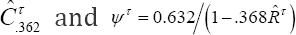 for the .632+ bootstrap cross validation estimate
  [5]. The relative over fitting rate
  is:
is:
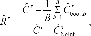
Where, ĈTNoInf corresponds to the no-information error rate of the restricted concordance probability for which the survival status is independent from the covariates x. As such, for each subject i of cluster j, its contribution to is computed by averaging over all the observed values of the data set or:
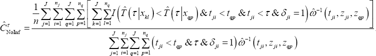
When is lower than 0 (higher than 1), is fixed to 0 (1). The .632+ bootstrap cross validation estimate will differ more from the .632 bootstrap cross validation estimate as Rt gets closer to 1. Further, [11] have found that the .632+ bootstrap cross validation estimate performs generally better than the .632 bootstrap cross validation estimate. An estimate of the frailty term of each of the clusters of the data set is needed to estimateCTBC However, it is possible that some clusters of the original data set are not present in the training set of step a) of the above procedure such that in the validation set of step c) no point estimates can be calculated for these subjects. Therefore, we propose to calculate CTBC in step c) only for those subjects whose cluster was present in the training set of step a). Note that it is assumed thatCTBC cannot be calculated for only a minority of the clusters of the validation data set such that the 63.2/36.8 proportion (training/validation) is not too strongly disrupted.
A too strong disruption of this proportion invalidates the upper internal validation scheme. A credible/confidence interval for the internally validated point estimate can be constructed by combining the above procedure and the one of Section 2.2.4. More specifically, we start by samplingK bootstrap data sets. For each of these bootstrap data sets, the upper procedure is repeated resulting in K validated measures  with k = 1.....,k. These validated measures are then used to construct a 95% credible/confidence interval by applying step e) of the procedure of Section 2.2.4.
Results
Simulation study
After describing the design of the simulation study, the properties of the Bayesian/likelihood point estimates and the percentile credible/confidence intervals of CTBC CTBM and CTW of the parametric failure time model are presented. In Section C of the online supplementary material, a full description of additional investigations is provided. Below we only report the conclusions of the additional investigations. These additional investigations entail the effect of changing the intra-cluster correlation, Changingτ and increasing the sample size on the Bayesian/likelihood point estimates of CTBC CTBM and CTW Also, the properties of the BCα credible/confidence intervals of the parametric failure time model and the properties of the Bayesian/likelihood point estimates of the semi-parametric failure time model of all measures are shown in Section C of the online supplementary material as well as the fitting procedures of the Bayesian/likelihood parametric and semi- parametric failure time model. This simulation study is repeated for the CT (d) measures detailed in Section D of the online supplementary material. Below we only report the conclusions of the latter simulation study.
Design of the simulation study
In this section we provide details on the simulation study. A gamma frailty proportional hazard (PH) model with a Weibull baseline hazard (shape ρ = 2, scale λ = 2.236 ) was chosen as the failure time distribution. Two subject-specific covariates were considered, each covariate was sampled from a standard univariate normal distribution. The β parameters were taken as (-2.45, 2.4), representing a population with strong covariate effects. All clusters are equal in size with cluster sizes 2, 5, 10 and 20. The variance parameter of the gamma frailty distribution equals 1 representing a population with a relatively large unobserved heterogeneity. This results in 4 different populations and for each of these populations censoring times are generated from a uniform distribution U (0,v) with chosen to obtain a censoring percentage of 0%, 25%, 50% or 80%. This leads to 16 scenarios for which the performance of CTBC CTBM and CTW (withτ equal to 1) is evaluated. For each of the scenarios, 100 (500) data sets of size 1000 were necessary for the estimation of the bias and MSE (coverage probability) to obtain stable results. All population parameters are chosen such that the covariates have an appreciable effect on the failure time distribution.
In order to evaluate the properties of CTBC CTBM and CTW the true values CTBC CTBM and CTW are computed empirically in the absence of censoring by sampling a large data set (N = 20,000) from each of the 4 populations and by calculating the CTBC CTBM and CTW using the true values of the parameters of the failure time. The fitted failure time model of the parametric model corresponds to a PH model with a Weibull baseline hazards. The fitted failure time model of the semi-parametric model corresponds to a classical Cox PH model with a partial likelihood estimation procedure [12] for the likelihood procedure and to a gamma independent increments model for the baseline hazards and a PH specification for the covariates [13] for the Bayesian procedure. Since no covariates influence the censoring process, the Kaplan-Meier model of [14] is chosen as the censoring model for the likelihood procedure and the gamma-independent increments model of [13] for the Bayesian procedure. The empirical bias is calculated as the averaged difference between the true and the estimated concordance probabilities and the MSE as the mean of the squared differences between the true and estimated concordance probabilities. A positive (negative) empirical bias is defined as any estimate greater (smaller) than the true value of CTBC CTBM and CTW respectively.
Simulation results for the parametric and semi- parametric model
Bayesian procedure: For the parametric model, no substantial empirical bias is seen over the different settings and that for all measures. The empirical MSE of CTBC (CTW) increases mildly as the cluster size increases (decreases), attaining considerably higher levels for a censoring percentage of 80% and a cluster size of 2. For all measures the empirical MSE increases slightly as the censoring percentage increases ( Figure 1 ). For CTBC and CTBM the estimated 95% coverage probability approaches the nominal level for all scenarios. For cluster sizes 2 and 5 (10 and 20), CTW attains an estimated coverage probability of about 98% (95%) (Table 2). For CTBC(CTBM and CTW ), the size of the credible interval increases as the cluster size increases (decreases) and/or the censoring percentage increases (Table 3). For the semi-parametric model,CTBC shows good estimation properties for the scenarios of a cluster size of 20 only. CTBM and CTW are virtually unaffected by the censoring percentagelind the cluster size.


Likelihood procedure: For the parametric model, CTBC shows a positive empirical bias which increases as the cluster size decreases and the censoring percentage increases. For CTBM and CTW no substantial empirical bias is seen over the different settings. The empirical MSE of CTBM and CTW increases as the cluster size decreases, and for all measures the empirical MSE increases as the censoring percentage increases, attaining significantly higher levels for a censoring percentage of 80% (Figure 2). For CTBM and CTW the estimated 95% coverage probability approaches the nominal level for all scenarios. For cluster sizes 2 and 5 (10 and 20), CTW attains an estimated coverage probability of about 98% (95%) (Table 2). For CTBC (CTBM, and CTW), the size of the confidence interval increases as the cluster size increases (decreases) and/or the censoring percentage increases (Table 3). The semi-parametric likelihood approach shows a similar behavior as the parametric likelihood approach.
Additional simulation results for the parametric model
The estimation ofCTBM by the Bayesian method shows no significant empirical bias, except when the intra-cluster correlation is very small, the cluster size very small and the censoring percentage very high. The latter empirical bias is provoked by an overestimation of the frailty variance parameter. For the likelihood method, CTBM shows a positive empirical bias which increases as τand the intra-cluster correlation increases, but which is unaffected by the sample size. The estimation properties of<CTBM and CTW by the Bayesian and likelihood method are not influenced by r, the intra-cluster correlation or the sample size. The quality of the credible/ confidence intervals of the percentile and BCα the bootstrap method are found to be very similar. Note that the estimate of the acceleration αT of the BCα non-parametric bootstrap method was found to be very small in every investigated scenarios, such that we recommend to fix the αT to zero.
Simulation results for the cT(d) measures
For the Bayesian method, similar properties for allcT(d) measures are found as for their corresponding cT measures. For the likelihood method however, an additional (negative or positive) empirical bias is observed for cTW(d) and CTBM(d) that increases as the censoring percentage increases. Note that this additional empirical bias is caused by the ϕ(.) weights since it requires the estimation of the conditional survival probability of the true failure time model. Indeed, the latter estimates are constructed by means of the empirical Bayes estimates of the frailty terms which will induce in some scenarios a positive empirical bias and in other scenarios a negative empirical bias. The estimation of cT(d) measures by means of the likelihood and Bayesian semi-parametric failure time model is only reliable for a sufficiently large cluster size (for a cluster of size 20 in our simulation study) and, for the likelihood method only, when the censoring percentage is not high (up until a censoring percentage of 25% in our simulation study).
Effect of misspecification
In this section, we show the effect of misspecifying the frailty distribution and the censoring model on the estimation properties of CTBC CTBM, and CTW the conclusion of these investigations is reported below, a full description of the simulation study and corresponding results can be found in Section E of the online supplementary material. Moreover, just the results of the Bayesian method are reported here since similar results are found for the likelihood method. For the latter method only an additional positive bias for CTBC is observed which increases as the cluster size and/or censoring percentage and/or degree of misspecification increases. This simulation study is also repeated for the cT(d) measures. For a full description of the latter simulation study and its results, we refer to Section F of the online supplementary material.
Misspecification of the frailty distribution
CTBMand CTW are virtually unaffected by misspecification of the frailty distribution. CTBC however, is in general strongly affected by misspecification, resulting in a positive (negative) bias when the empirical distribution of the estimated frailty terms Ŵ is more (less) variable than the distribution of the true frailty terms W. Similar results were found by [15].
Misspecification of the censoring model
A functionally misspecified covariate effect or a misspecified censoring model will result in a negative bias, especially for high censoring percentages (50% and 80% in our simulation study). Covariates that have no impact on the censoring process will not influence the quality of the estimation when included in the censoring model. Omitting important variables, however, does result in a negative bias. In practice, several equally performing censoring models can be proposed. This is however not a problem since the censoring model is merely used as a working model. Note however it is easier to detect misspecifications of the censoring model as the censoring percentage increases since, in contrast to the failure time model, a higher censoring percentage results in an increase of information for the censoring model. Similar results were found by [16].
Simulation results for the CT(d) measures
Due to the misspecification of the frailty distribution, the estimated frailty terms differ from the true frailty terms, hereby not only disrupting the bias patterns of CTBC (d), but also of CTBM(d) and CTW(d) since the estimated frailty terms are also used in the calculation of the ϕ(.) weights. We therefore recommend to use CT(d) the measures only to appreciate a good fitting model in more detail. The results of the misspecification of the censoring model are very similar to what was obtained for the CT measures.
Application to the amalgam data set
In this data set, the effect of different treatment modalities on the longevity of different types of amalgam restorations is investigated. The primary covariates of the study are 4 cavity wall treatments ('CSA', 'CWF', 'Copalite' and 'Silver Suspension') and the alloy of the amalgam (levels: 'NTD', ‘Tytin’ and 'CNG'). The secundary covariates are the type of the restoration (levels: 'MO/DO' and 'MOD'), the type of tooth (levels: 'premolar’ and 'molar'), the position of the tooth in the mouth (levels: 'upper left', 'upper right', 'lower left' and 'lower right'), the operator (levels: 'operator 1', 'operator 2’ and 'operator 3’), gender and age. The data set is composed of three clinical trials and in each clinical trial the primary variables were combined into 4 treatment modalities assigning each modality randomly to 4 (or 8 or 12) teeth in a 2 x 2 (factorial) design within patient [17]. Note that this study was mainly designed to evaluate significance of the primary covariates. In this paper we will evaluate the predictive potential of all the primary covariates. Since the early failures are suspected to be of a different nature than the late failures and since there are only a few early failures, we restrict our analysis to the late failures only, i.e. failures that occur at least 9 years after enrollment in the study. This results in 174 patients contributing with 1347 amalgam restorations. The clustered data structure is unbalanced, with 4, 8 and 12 restorations seen in 36, 89 and 33 patients, respectively. The median follow-up time is 14.48 and the true failure time is observed for 187 amalgam restorations only, leading to a censoring percentage of 86.2%.
Based on the results of the simulation studies of Section 3.1, we have chosen to use the Bayesian gamma frailty generalized gamma model as the failure time model, which is a very flexible parametric Bayesian model [18]. Note that the failure time model consists of the primary covariates only. Different censoring models for the IPCW weights were tested with the Bayesian generalized gamma model of both primary and secondary covariates resulting into the highest concordance probability estimates. We evaluate the model's discriminatory ability from 9 to 15 years after enrollment in the study, since, as recommended by [19], censoring is not too heavy at the end of this time interval. The +.632 bootstrap cross validation estimators are chosen for the internal validation of the considered concordance probabilities. The R code of this analysis but applied to fictive data can be found in the online supplementary material.
Analysis using the full information
The apparent and validated point estimate and 95% percentile credible interval of the Cτ measures (B = 100, K = 100, τ = 6 ) are shown in Table 4. Since r is chosen to be 6, all comparable pairs of the [9,15] time interval are considered. Little difference with the values in Table 4 is found for CT (d) measures using τ = 6 We see that the covariates have practically no intra-cluster predictive ability but a strong inter-cluster predictive ability. Further, even after validation, the between conditional concordance probability improves reasonably strongly on the between marginal concordance probability implying the presence of a strong clustering effect upon the covariate effects. Thus, if one succeeds in a future study to fully capture the clustering effect in covariates and if the primary variables are also included in this future model, the between marginal concordance probability can potentially attain a value of 0.74. Note that the drop in predictive ability due to the internal validation is more pronounced for the between conditional concordance probability than for the between marginal and within concordance probability. All the apparent and validated 95% percentile credible intervals show a strong overlap and the upper bound of the validated 95% percentile credible intervals are all lower than the upper bound of the apparent 95% percentile credible intervals. Surprisingly, the lower bound of the validated 95% percentile credible intervals of the within and the between marginal measures are higher than the upper bound of the apparent 95% percentile credible intervals.

Analyzing τ and d- varying patterns
In Figure 3, the apparent and validated time-varying CT and CT (d) estimates are shown. In the left panel of Figure 3, no CT estimates are available for a τ value lower than 10.2. Indeed,CT can only be estimated when at least one true failure time has been observed prior to t, which is only the case from 10.2 years onwards. Further,CTBC ( CTBM and CTW ) attain lower (higher) values as T increases, implying that early failing teeth are easier (more difficult) to discriminate from later failing teeth than later failing teeth are. As a result, the difference between the validated curves of CTBC and CTBM mildly decreases as τ increases such that the clustering effect induces a stronger gain in predictive ability for the earlier failing teeth as compared to the later failing teeth. Note thatCTW even attains values lower than 0.5 for τ values lower than 14, meaning that the ranking of the predictions are systematically in the wrong direction for teeth belonging to this τrange. In the right panel of Figure 3, a monotone increasing pattern is depicted for both CTBCand CTBM (d)The validated patterns of both measures exceed 0.5 only for d values higher than 0.7 and remain to be very similar up until a d value of 1. Stable results are obtained for CTBC (d) once d exceeds 3 years. This means that the clustering effect only increases upon the predictive ability of the covariates for inter-cluster pairs with a difference in failure time of minimum 1 year and of maximum 3 years. The validated pattern of CTW approaches a straight line and reveals an almost complete absence of intra-cluster predictive ability of the primary covariates for this data set.

Discussion
In this article, the methodology proposed in [1] is extended to general frailty models. Also, a new definition of the concordance probability is developed as well as an internal validation procedure and a procedure to calculate interval estimates in the presence of clustered data. Note that all these developments can also be applied to univariate survival models, we just focused on the frailty model in this article. Other very useful measures can be extended to the frailty model in a similar manner [19-22]. We chose the concordance probability since it is most widely used measure for the discriminatory ability of survival data. From the simulation study, we learned that it is of mayor importance to model the censoring model correctly. Despite of this possible shortcoming, the IPCW estimation method is up to now, to our knowledge, the best method to estimate the concordance probability in the presence of censoring. An alternative estimation method could be based on a non-parametric imputation method based on the covariate distribution, in which the censored failure times are replaced by true failure times whose covariate information is close to the one of the censored observation. This estimation would be, in spirit, similar to what has been done by [23] for the estimation of survival models.
The between conditional concordance probability estimated by the likelihood approach suffers from a negative bias, especially for a small cluster size and a high censoring percentage. By means of a small simulation study, we could determine that this overoptimistic bias is caused by the empirical Bayes estimates of the frailty terms since the overoptimistic bias of the between conditional concordance probability disappeared once the frailty terms were replaced by their population values. Note that similar results were found in [1] and [24]. An external validation of the between conditional concordance probability can only be performed when the same clusters are used for the external data set as for the training data set. Indeed, only under these conditions estimates of the frailty terms for the clusters of the external data set are available, indispensable to compute the between conditional concordance probability of the external data set. Note that this only emphasizes the importance of an internal validation procedure for the between conditional concordance probability. A different solution to this problem could be the estimation of the frailty term of a new cluster, but this approach was not considered here. In this article we extended the concordance probability for frailty models with a 2-level clustering structure, since this is the most common clustering structure in survival analysis [7]. In practice however, more complicated clustering structures may be encountered. In [24] for example, it is shown how the concordance probability and the Brier score can be extended for nested 2-level and 3-level multilevel binary regression models.
Acknowledgement
The authors would like to thank Cees Kreulen for the permission to use the amalgam data set [17] for this research. For the computations, we used the infrastructure of the VSC - Flemish Supercomputer Center, funded by the Hercules Foundation and the Flemish Government - department EWI. Support from the IAP project Phase VII (P07/6, 2012-2017) to develop crucial statistical methods for understanding major complex dynamic systems in natural, biomedical and social sciences from the Federal Office for Scientific, Technical and Cultural Affairs of Belgium is gratefully acknowledged.
References
- Van Oirbeek R, Lesaffre E (2010) An application of Harrell's C-index to PH frailty models. Stat Med 29(30): 3160-3171.
- Gerds TA, Kattan MW, Schumacher M, Changhong Y (2013) Estimating a time dependent concordance index for survival prediction models with covariate dependent censoring. Stat Med 32(13): 2173-2184.
- Heagerty PJ, Zheng Y (2005) Survival model predictive accuracy and ROC curves. Biometrics 61(1): 92-105.
- Maugain A, Collette S, Pignon JP, Rondeau V (2013) Concordance measures in shared frailty models: application to clustered data in cancer prognosis. Stat Med 32(27): 4803-4820.
- Gerds TA, Schumacher M (2007) Efron-type measures of prediction error for survival analysis. Biometrics 63(4): 1283-1287.
- Harrell Jr FE, Califf RM, Pryor DB, Lee KL, Rosati RA (1982) Evaluating the yield of medical tests. J AMA 247(18): 2543-2546.
- Duchateau L, Janssen P (2008) The Frailty Model. Springer Science + Business Media, New York, USA.
- Efron B, Tibshirani RJ (1993) An Introduction to the Bootstrap. Chapman & Hall/CRC: London, Boca Raton, FL, USA.
- Field CA, Welsh AH (2007) Bootstrapping clustered data. JR Statist Soc B 69(part 3): 369-390.
- Rubin DB (1981) The Bayesian bootstrap. The Ann Statist 9(1): 130134.
- Efron B, Tibshirani RJ (1997) Improvements on cross-validation: the .632+ bootstrap method. Journal of the American Statistical Association 92(438): 548-560.
- Cox DR (1972) Regression models and life-tables. Journal of the Royal Statistical Society, Series B (Methodological) 34(2): 187-220.
- Kalbfleisch JD (1978) Nonparametric Bayesian analysis of survival time data. Journal of the Royal Statistical Society, Series B 40(2): 214221.
- Kaplan EL, Meier P (1958) Nonparametric estimation from incomplete observations. Journal of the American Statistical Association 53(282): 457-481.
- Glidden DV, Vittinghoff E (2004) Modelling clustered survival data from multicentre clinical trials. Stat Med 23(3): 369-388.
- Gerds TA, Schumacher M (2006) Consistent estimation of the expected Brier score in general survival models with right-censored event times. Biom J 48(6): 1029-1040.
- Kreulen CM, Tobi H, Gruythuysen RJM, van Amerongen WE, Borgmeijer PJ (1998) Replacement risk of amalgam treatment modalities: 15-year results. J Dent 26(8): 627-632.
- Cox C, Chu H, Schneider MF, Munoz A (2007) Parametric survival analysis and taxonomy of hazard functions for the generalized gamma distribution. Statistics in Medicine 26(23): 4352-4374.
- Graf E, Schmoor C, Sauerbrei W, Schumacher M (1999) Assessment and comparison of prognostic classification schemes for survival data. Stat Med 18(17-18): 2529-2545.
- Schemper M, Stare J (1996) Explained variation in survival analysis. Stat in Med 15(19): 1999-2012.
- O Quigley J, Xu R, Stare J (2005) Explained randomness in proportional hazards models. Stat in Med 24(3): 479-489.
- Pencina M, DAgostino Sr RB, DAgostino Jr RB, Vasan RS (2008) Evaluating the added predictive ability of a new marker: From area under the ROC curve to reclassification and beyond. Statistics in Medicine 27(2): 157-172.
- Hsu CH, Taylor JMG, Murray S, Commenges D (2006) Survival analysis using auxiliary variables via non-parametric multiple imputation. Stat Med 25(20): 3503-3517.
- Van Oirbeek R, Lesaffre E (2012) Assessing the predictive ability of a multilevel binary regression model. Computational Statistics & Data Analysis 56(6): 1966-1980.


