


Weibull Analysis for Constant and Variant Stress Behavior Using the ALT Method for Single Stress and the Taguchi Method for Several Stress Variables
Manuel R Piña Monarrez*
1Department of Industrial and Manufacturing, Universidad Autónoma de Ciudad Juárez, México
Submission: January 22, 2018; Published: April 18, 2018
*Corresponding author: Manuel R Piña Monarrez, Department of Industrial and Manufacturing, Engineering and Technological Institute, Universidad Autónoma de Ciudad Juárez, México; Email: manuel.pina@uacj.mx
How to cite this article: Manuel R P M. Weibull Analysis for Constant and Variant Stress Behavior Using the Alt Method for Single Stress and the Taguchi Method for Several Stress Variables. Biostat Biometrics Open Acc J. 2018; 6(2): 555681. DOI: 10.19080/BBOAJ.2018.06.555681.
Abstract
The article presents the advances on Weibull analysis which let practitioners to plan the data collection test, to fit the Weibull parameters directly from the applied stress values, to determine the capability indices cp and cpk, and to formulate the control charts to monitor the Weibull parameters. Thus, the theoretical background and formulation as well as numerical examples for constant and variant stress behavior are given. Also the references where the discussed methods were mathematically formulated and numerically applied are provided.
Keywords: Weibull demonstration test plan; Accelerated life time analysis; Taguchi method; Sample size; Capability indices
Abbreviations: NHPP: Non-Homogenous Poisson Process; T: Temperature; ALT: Accelerated Life Time Data; Mn: Manganese; Mg: Magnesium; HMPC: Hot Mill Pass Counts; CMR: Cold Mill Reduction Rate
Introduction
Since the Weibull distribution is the best probability density function (pdf) used to model the behavior of a quadratic form [1,2], as they are any response surface model [3], the stress and strain matrix used in mechanical and structural analysis [4], the covariance matrix used in principal component analysis [5], and the branching process behavior [1]. Then an understanding of the Weibull distribution features is needed. Based on the above, this paper presents the advances on Weibull analysis to perform it from the planning data collection phase to the monitoring process phase. Therefore, the papers' structure is as follows. In section 2, the general new background of the Weibull distribution and the formulation to determine the sample size to perform a zero failure Weibull demonstration test plan are presented. In section 3, the formulation to determine the capability cp and cpk indices and the formulation of the control charts which let us to monitor the estimated Weibull parameters are given. In section 4, the formulation to fit the Weibull shape pand scale n parameters directly from the applied stress values is presented. In section 5 a numerical example for constant stress is given. In section 6 a numerical example for variant stress is given. Finally, in section 7 the conclusions are presented. The analysis is as follows:
Weibull distribution background and sample size
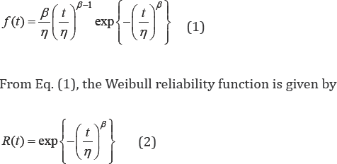
The two parameter Weibull distribution [6] is given by
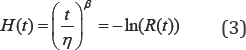
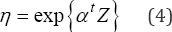
And since the Weibull distribution is generated by a non- homogenous Poisson process (NHPP) [7] sec 4.3, then the Weibull risk function depends on the time also. Thus, the mean power function of the related NHPP in Weibull analysis is used as the cumulative hazard risk function H(t)? From Eq. (2), h(t). is given by
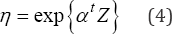
In Weibull analysis Eq. (3) is of special interest because for the desired time t and known p value the effect that the stress variable s has on the estimated R(t) index is given by the linear relationship between n and s as
In Eq. (4), a is a regression coefficient vector a = [Kp, .,pp} and Z is a nxp matrix which contains the k stress variables (Sj,s2,...,sk) and p represents the k variables effects plus the possible effects generated among the k variables (e.g. interaction and quadratic effects). Also note from Eq. (2), that for known t and p values, the n value which corresponds to a desired R(t) index is completely addressed and it is given as
On the other hand, because by setting H(t)=1 in Eq. (3) the sample size n which have to be tested to accurately estimate 1, was derived in [8]. as
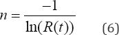
Then, from Eq. (5 and 6) 1 in terms of n is given by
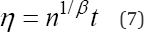
Eq. (6) is too important in Weibull analysis because by using it in Eq. (7), then value which corresponds to any feasible or desired t (t > 0), P(P> 0) andR(t) values is completely determined without any experimentation or observed lifetime data. As an example suppose we desire to determine the value which corresponds to R(t)=0.9535 for t = 1500hrs and p = 3. Thus from Eq. (6) n=21 and by using it with p = 3. and t = 1500hrs in Eq. (7), n = 211/31500 = 4i38.38hrs. Hence, because the value estimated in Eq. (6) completely determine , then this n value also represents the sample size which has to be tested without failures in order to accurately estimate the minimum n value for which the tested element will present at least the desired reliability index. As a simple example suppose we have to demonstrate a product fulfills with R(t) = 0.95 for t = 1500hrs Thus, because from Eq. (6) n = 19.4957, then 19 parts has to be tested by 1500hrs each and one part has to be tested by 0.4957(1500)=743.595hrs. It is to say, n in Eq. (6) is not a discrete value, instead it is continuous and it represents the times the desired time t has to be tested in order to demonstrate the tested product fulfills at least with the desired R(t) index. Now we know n in Eq. (6) represents the right sample size to design a zero failure Weibull demonstration test plan, let present the capability indices and the corresponding control charts.
Weibull capability indices and control charts
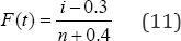
When the Weibull analysis is being performed for example in the quality field or in an improvement process, the related capability index cp and ability index cpk are of interest. Fortunately by using the log-mean(mx) and the log-standard (^x) deviation parameters of the observed (or expected) failure times, as was demonstrated in [9] and [10], the Weibull cp and cpk indices can both be estimated. In particular, they are formulated based on the direct relationships between the Weibull p 1 parameters with the log and parameters. These relationships are
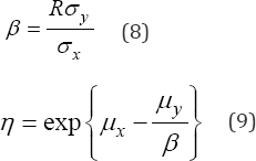
In Eq. (8), R is the multiple correlation coefficient between the responses Yi values and the logarithm of the failure times (Xi =ln (ti)) (here after, by supposing data is Weibull, R = 1). In Eq. (9) My and in Eq. (8) oy are the mean and the standard deviation of the response vector given by

In Eq. (10),b0 and B are parameters to be estimated and the cumulated failure probability (F (t,)) is given by the median rank approach here approximated by the well-known Bennard formula as
Therefore, based on the oy parameters given in Eqs.(8 and 9), the corresponding cp and cpk indices are
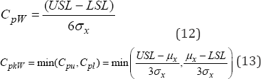
In Eq. (10 and 11), USL and LSL are the upper and lower product's specifications limits measured in time units. And if they are unknown, then the minimum and maximum expected lifetimes of the Weibull analysis can be used to estimate them. These maximum and minimum lifetimes are estimated from Eq. (10) by using the Yn maximum element to estimate the maximum lifetime and by using the Yt minimum element to estimate the minimum lifetime as

On the other hand, based on the facts that
1) In Weibull analysis theR (t) index is completely defined by the β and V parameters, and
2) The � and � are determined by the ()x�[Eqs. 8 and 9].
Then in [12], the Weibull control charts to monitor p and n were formulated by setting (ctJ as the upper control limit to monitoring. And by setting (ft) as the lower control limit to monitoring n. Here it is too important to highlight because represent the central parameters in logarithm scale, then in the case where we are analyzing several variables can be estimated by using the Taguchi method as it is made in [11]. And of course, once they had been already estimated, they can be used in Eqs. (8 and 9) to estimate the corresponding p and n parameters, as well as in Eqs. (12 and 13) to determine the corresponding capability indices; for details see [12]. Now let present how to estimate p and 1 directly from the applied stresses values.
Estimation of p and ij directly from the stresses values
Since in Weibull analysis p and 1 completely determine the estimated R(t) index, and because p represents the aging of the analyzed system, then their accurate estimation is needed. Fortunately, as demonstrated in [4] both p and rj can be directly estimated from the maximum and minimum applied stresses values. The estimation is made by using the eigen values of the analyzed quadratic form as the maximum and minimum applied stress values. As examples of quadratic forms suppose we are analyzing a biological phenomenon by using a response surface model given by

Thus, its quadratic form is 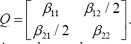 Similarly suppose from the stress analysis we know the normal stresses and the shear stress xy� values. Hence, the stress
quadratic form is  As a third example of quadratic form suppose in a principal component (pc) analysis we know the variance and the covariance among the variables. Thus, the
pc quadratic form is 1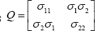 Therefore based on [4], by using the eigen values λ1 and λ2 of the quadratic form Q,the β value is given as
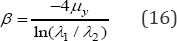
In Eq. (16) μy is the mean of the response vector defined in Eq. (10). And because the log-mean is directly given as the square root of the determinant of the Q matrix (for details see sec. 2.2 in [4]), then by using y� and the estimated μ values in Eq.(9),� is directly estimated. It is to say from Eq. (16) � is estimated and from Eq. (9) the corresponding � value is estimated. Now let present the numerical examples.
Numerical example for constant stress behavior
In this section two numerical example with constant stress behavior are presented. In the case of single stress variable, the temperature (T) is used as the stress variable. And for several stress variables the Taguchi method is used.
Analysis with a single stress variable

In this section let used data published in [13]. The 10n=collected lifetimes are given in Table 1. Data corresponds to an accelerated life time data (ALT) subjected to a single stress variable (temperature in Kelvin degrees). The normal level is 323NK= and the accelerated levels are lower 393,LK= middle 408MK= and higher 423.HK= Thus, because data of Table 1 is an ALT data, then first the � parameter of the normal level 323TK= has to be determined. And because the stress variable is a fixed temperature value, then the life/stress Arrhenius models is used. (If the stress is a range of temperature, then the Coffin Mason model should be used). The Arrhenius model ([14] sec.5.5.1) is given as
In Eq. (17) C and B are parameters to be estimated. Thus, by using Eq. (1) and Eq. (17) in the ALTA software, the estimated Arrhenius parameters are p = 4.2916, C = 58.9848 and B = 1861.6187. As a consequence, by using the estimated C and B values with T=323 in Eq. (17), the normal scale parameter is n = 18784.83^rs. Therefore the Weibull distribution of the normal setting is W(4.2916, 18784.83). On the other hand, the values which corresponds to R(t)=0.9535 are estimated by using fty =-0.545624 and ay = 1.1751169. were estimated by using r (t ) = 1 - f (t ) = 0.9535 in Eq.(10)
Therefore, from Eq. (9), ft =9.7136675 and from Eq. (8) oy= 0.2738179. And because n = -1/ln (0.9535) = 21, then Yn = ln (-ln (1 -((21 - 0.3^21.4))) = 1.22966, Y1 =-3.403483. Thus, from Eq. (14) UCL= 10.12733 and LCL=9.04774. And as a consequence from Eq.(12), cpw=0.657118. And from Eq. (13) cpkw=min(0.5035, 0.8106)=0.5035.. Finally, ^ = 02738179 has to be set as the maximum allowed value to monitor p. Similarly = 9.7136675 has to be set as the lower allowed value to monitor n. Now let present the multivariate analysis.
Analysis with several stress variables
In this section, the analysis is based on [11]. The used data given in Table 2 was first published in [15]. The analyzed factors were the aluminum-alloy content in manganese (Mn) and magnesium (Mg) as well as hot mill pass counts (HMPC) and cold mill reduction rate (CMR). Mn, Mg, and CMR were measured in percentage units until dome yielded 1mm on a constantly applied external pressure of 500psi. From the Taguchi analysis ([11] sec.3.3.2) the robust level is Mn=1.6, Mg=1.8, HMPC=35, and CMR=30. The found robust's log-parameters are nx = 3.5442 and nx = 0.024141. Thus, from Eq.(8) p = 40.82715 and from Eq.(9) n= 35.0307.

On the other hand, because in the monitoring process the variables which determine the values are the process variables which have to be monitored. And because in order to correctly monitor the contribution that each variable has on the observe values have to be determined, then their contribution have to be determined also. Fortunately because nx is directly given from the determinant of the Q matrix as it is made in [4], then the decomposition method given in [19] can be used to determine the mentioned variable contributions. Also it is important to mention that the mathematical formulation to determine the value and the variables which determine its value, can be performed by partitioning the Q matrix as it is made in [20]. Finally the value to monitor p = 1.847127 is determined by using ay =11751169 in Eq. (8). The (°x) value to be set in the corresponding chart as the maximum allowed value is ax = 0.636186. And because n = 3126.926895 and ft =-0.545624, then from Eq. (9) the value to be set in the corresponding chart as the minimum allowed value to monitoring 1 is ftx = 8.343197.
Numerical example for constant stress behavior
In this section two numerical example with variable stress behavior are presented. In the first case data published in [4] is used to show how a product can be designed. In the second case data published in [17] is use to show how the ALT analysis can be used to analyze variable stress behavior. The analysis is as follows
Variable stress analysis focused on product's design
In this section the focus is on product's design. The analysis is performed following [4]. The objective consists on determining the R (t) index of a mechanical or structural design subjected to the normal stresses ax =and a shear stress Txy = 40mpa. Thus, as mentioned in section 4, the stress matrix Q which model the variant stress behavior is
From the Q matrix, the principal stresses or eigen values are <7j = \2H2mpa and u2 = 42.28mpa. And as a consequence, the principal stress behavior is in the interval [42.28 - \27.72] mpa. And because in [4] R (t ) = 0.9535 was used, then from the Yi elements generated in Eq. (10), their mean is ny =-0.545624 and their standard deviation is oy = \.\75\\69. Hence, by using the P, value and the and ct2 values in Eq. (16), the estimated Weibull shape parameter is P = \.984693. And by using the °y and P values in Eq. (8), = 0.592090. Finally, because from the logarithm of the square root of the determinant of the stress matrix Q, Px = 4.29707726, then from Eq.(9), the Weibull scale parameter is n = 9673676mPa. Therefore the addressed Weibull family is W(1.984693, 96.7367). However, because in variable stress analysis, the stress variable instead of be a single value it is a range of stress values, then the addressed Weibull family only represents the stress distribution which models the stress range behavior as shown in Table 2 in [4]. As a consequence, in order to determine the R (t ) index of the analyzed product, the Weibull distribution which models the strength of the product to overcome the applied stress has to be determined. In [4] sec. 4.4.2, because the used material strength was sy=400mpa, then the addressed strength Weibull family is W(1.984693, 455.2318). Finally, by using both the stress and the strength distributions in the Weibull/Weibull stress/strength methodology ([18] chapter 4 to 6), the stress/strength R (t ) index is given as
In Eq. (18) P = 1.984693, n = 96.73676 and ns = 455.2318. As a consequence, the addressed stress/strength R (t ) index is R (t ) = 95.58. It is to say a product designed with sy=400mpa performing in a variant stress range of [42.28, 127.72]mpa will present a R (t ) = 95.58. [4].
On the other hand, although in variable stress analysis the cp and cpk indices defined Din Eqs. (12 and 13) are not defined for the Weibull/Weibull stress/strength function yet, the related control charts can be used to monitor the stress and the strength Weibull parameters. Thus, ax = 0.592090 should be used as the maximum value to monitor the common p value, and ftx = 4.29707726 should be used as the maximum value to monitor the stress n value. Also observe because here represents the stress distribution it was set as the maximum allowed value. On the other hand, when it represents the strength distribution, it should be set as the minimal allowed value. Finally, the value to monitor the strength Vs value is determined by using ft =-0.545624, p = 1.984693 and nS = 455.2318 in Eq. (9). The estimated value to be monitored as the minimal allowed stress value is ft = 5.845891. Now let present the stress variable case using ALT data.
Variable stress analysis by using ALT data
In this section the focus is to show how the ALT analysis can be used to analyze variable stress behavior. The used data was published in [17]. Data represents a set of 65 ball bearings tested at loads of 3500, 3800 and 4500 pounds. (Observe because the stress variable behavior by itself represents the normal stress behavior, then in the ALT analysis no extrapolation is needed). In the analysis the lognormal distribution with log parameters ft = 7.6 and ax = 0.4 were used to represent the stress variable behavior. And the Weibull distribution was used to represent the corresponding life times behavior of the ball bearings. From the collected 65 ALT data, the Weibull p parameter and the K and n parameters of the used inverse power model (IP)were estimated. The IP model [14] is given by
In Eq. (19), V represents the stress variable (pounds in this case). From the ALT analysis in [17], p = 1.847127, n=3.624360, and K=7.166599E-18. Then 21 stress values in the interval [1000, 4000] punds were selected, and by using them with the estimated IP parameters in Eq. (19) 21 values were predicted. Then by using p= 1.847127, and the 21 estimated n values in Eq. (2), the corresponding R(t) indices for t=30000 were estimated and used in Eq. (10) to determine the corresponding 21 Yt elements. Finally by using the logarithm of the 21 stresses values and the estimated 21 Yt elements, in a regression, the Weibull parameters of the strength distribution were estimated. The fitted Weibull parameters of the strength distribution are p = 6.694655, and n = 3126.926895. Therefore, the addressed Weibull strength distribution is W(6.694655, 3126.926895). Here it is too important to observe the addressed Weibull family only represents the behavior for fixed t=30000, if other t value is desired the above process has to be repeated [17]. Finally, by using the lognormal stress distribution and the Weibull strength distribution in the lognormal/Weibull stress/strength analysis [18], the corresponding R(t) index was determined. The found R (t) index is R (t ) = 0.7954; [17].
On the other hand, although the cp and cpk indices are not defined for the lognormal/Weibull stress/strength analysis yet, the monitoring process of the addressed stress and strength parameters can be performed. This can be done because both the lognormal and the Weibull distribution are based on the log parameters. Therefore the lognormal parameter ftx = 7.6 can be monitored by set ft = 7.6 as the maximum allowed stress level in a control chart. Note it was set as the maximum because it represents the stress distribution. It is to say, because In the stress/strength analysis the higher the stress value the lower the R(t) index then it has to be set as the maximum allowed value. Similarly, the log normal parameter can be monitored by using ax = 0.4 as the maximum allowed value also [18].
On the other hand, because in the monitoring process the variables which determine the values are the process variables which have to be monitored. And because in order to correctly monitor the contribution that each variable has on the observe values have to be determined, then their contribution have to be determined also. Fortunately because nx is directly given from the determinant of the Q matrix as it is made in [4], then the decomposition method given in [19] can be used to determine the mentioned variable contributions. Also it is important to mention that the mathematical formulation to determine the value and the variables which determine its value, can be performed by partitioning the Q matrix as it is made in [20]. Finally the value to monitor p = 1.847127 is determined by using ay =11751169 in Eq. (8). The (°x) value to be set in the corresponding chart as the maximum allowed value is ax = 0.636186. And because n = 3126.926895 and ft =-0.545624, then from Eq. (9) the value to be set in the corresponding chart as the minimum allowed value to monitoring 1 is ftx = 8.343197.
Finally, it is important to note the estimated stress/strength R (t ) = 0.7954 index was not used to estimate fty =-0.545624 and ay = 1.1751169 instead R (t ) = 0.9535 was used. This is made in this way because in the stress/strength analysis, the stress distribution is independent of the strength distribution. Therefore, the generated stress/strength function only represents the effect that all possible stress values have over the all possible strength values [18].
Conclusion
In this paper the advances on the theoretical interpretation of the features of the Weibull distribution which let practitioners to perform an integral analysis from the test planning phase to the monitor phase are presented. This is made based on the fact the Weibull distribution efficiently model a quadratic form. Among the more important features given in this article are?
The Weibull parameters p and V are completely determined from the maximum and minimum eigen values of the analyzed quadratic form (see sec. 4).
Because the addressed n value in Eq.(6) only depends on the desired R(t) index, then the estimated n value is robust under any uncertainties of the used t and p values; and in particular observe from Eq. (61) in [4] that because this n value also represent the base lifetime of any Weibull analysis, then Eq. (6) can be used to determine the expected lifetimes after any reliability improvement process.
The mean of the expected logarithm of the lifetimes is completely determined by the logarithm of the square root of the determinant of the analyzed quadratic form Q.
Although the Weibull cp and cpk indices are estimated by using the logarithm parameters because they are dimensionless they are efficient.
By monitoring the log-parameters the p and n parameters are completely controlled.
References
- Segun Goh, Kwon HW, Choi MY (2014) Discriminaring between Weibull distributions and log-normal distributions emerging in branching processes. J Phys A Math Theor 47: 22.
- Todinov MT (2009) Is Weibull the correct model for predicting probability of failure initiated by non-interacting flaws?. International Journal of solids and structures. 46(3): 87-901.
- George E P, Box, Draper (1987) Empirical Model Building and Response Surfaces. Wiley Series in Probability and Mathematical Statistics 13: 978-0471810339.
- Piña-Monarrez MR (2017) Weibull stress distribution for static mechanical stress and its stress/strength analysis. Qual Reliab Engng Int p. 1-16.
- Peña D (2002) Análisis de Datos Multivariantes. McGraw Hill/ Interamericana de España.
- Weibull W (1939) A statistical theory of the strength of materials. Proceedings, R Swedish Inst Eng Res 151: 45.
- Rinne H (2009) The Weibull distribution a handbook. Chapman and Hall/CRC press, Boca Ratón, FL, USA.
- Piña-Monarrez MR, Ramos LML, Alvarado IA, Molina ARD (2016) Robust sample size for weibull demonstration test plan. DYNA 2016 83: 52-57.
- Piña-Monarrez MR, Ortiz YJF, Rodriguez BMI (2016) Non-normal capability indices for the Weibull and lognormal distributions. Qual Reliaby Engng Int 32:1321-1329.
- Piña-Monarrez MR, Baro Tijerina M, Ortiz YJF (2017) Unbiased Weibull capability indices using multiple linear regression. Qual Reliaby Engng Int 33(8): 1915-1920.
- Piña-Monarrez MR, Ortiz YJF (2015) Weibull and lognormal taguchi analysis using multiple linear regression. Reliability Engineering and System Safety 144: 244-53.
- Piña-Monarrez MR (2016) Conditional Weibull control charts using multiple linear regression. Qual Reliab Eng Int 33(4): 785-791.
- Vassiliou P, Metas A (2002) Understanding accelerated life-testing analysis, Reliability and Maintainability Symposium (RAMS), Tutorials CD, Seattle, WA, USA.
- Bagdonavicius V, Nikulin M (2002) Accelerated life models, modeling and statistical analysis, Ed. Chapman and Hall/CRC, Boca Ratón, FL, USA.
- Besseris GJ (2010) A methodology for product reliability enhancement via saturated-unreplicated fractional factorial designs. Reliab Eng Syst Saf 95:742-749.
- Piña-Monarrez MR, Avila CC, Marquez LCD (2015) Weibull accelerated life testing analysis whit several variables using multiple linear regression, DYNA 82(191): 156-162.
- http://www.weibull.com/hotwire/issue172/hottopics172.htm
- Kececioglu D (2003) Robust Engineering Design-By-Reliability with Emphasis on Mechanical Components & Structural Reliability. DEStech Publications 1: 722.
- Piña-Monarrez MR (2013) Practical Decomposition Method for T2 Hotelling Chart. International Journal of Industrial Engineering Theory Applications and Practice 20(5-6): 401-411.
- Piña-Monarrez MR (2011) A New Theory in Multiple Linear Regression. International Journal of Industrial Engineering Theory Applications and Practice 18(6): 310-316.


