


Partial Variable Selection and Its' Applications in Biostatistics
Jingwen Gu1, Ao Yuan's1,2* and Ming T Tan1
1Department of Biostatistics, Bioinformatics and Biomathematics, Georgetown University, USA
2Department of Epidemiology and Biostatistics Section, Rehabilitation Medicine, National Institutes of Health, USA
Submission: December 23, 2017; Published: April 18, 2018
*Corresponding author: Ao Yuan, Department of Biostatistics, Bioinformatics and Biomathematics, Georgetown University, Washington DC 20057, USA; Email: ay312@georgetown.edu
How to cite this article: Jingwen Gu, Ao Yuan, Ming T Tan. Partial Variable Selection and Its� Applications in Biostatistics. Biostat Biometrics Open Acc J. 2018; 6(1): 555678. DOI:10.19080/BBOAJ.2018.06.555678
Abstract
We propose and study a method for partial covariates selection, which only select the covariates with values fall in their effective ranges. The coefficients estimates based on the resulting data is more interpretable based on the effective covariates. This is in contrast to the existing method of variable selection, in which some variables are selected/deleted in whole. To test the validity of the partial variable selection, we extended the Wilks theorem to handle this case. Simulation studies are conducted to evaluate the performance of the proposed method, and it is applied to a real data analysis as illustration.
Keywords: Covariate; Effective range; Partial variable selection; Linear model; Likelihood ratio test
Abbreviations : NIH: The National Institutes of Health; UPDRS: Unified Parkinson's Disease Rating Scale
Introduction
Variables selection is a common practice in biostatistics and there is vast literature on this topic. Commonly used methods include the likelihood ratio test [1], AIC [2], BIC [3], the minimum description length [4,5], etc. The principal components models linear combinations of the original covariates, reduces large number of covariates to a handful of major principal components, but the result is not easy to interpret in terms of the original covariates. The stepwise regression starts from the full model, and deletes the covariate one by one according to some statistical significance measure. May et al. [6] addressed variable selection in artificial neural network models, Mehmood et al. [7] gave a review for variable selection with partial least squares model. Wang et al. [8] addressed variable selection in generalized additive partial linear models. Liu et al. [9] addressed variable selection in semiparametric additive partial linear models.
The Lasso [10,11] and its variation [12,13] are used to select some few significant variables in presence of large number of covariates. However, existing methods only select the whole variable(s) to enter into/delete from the model, which may not the most desirable in some bio-medical practice. For example, in the heart disease study [14,15], there are more than ten risk factors identified by medical researchers in their long time investigations, with the existing variable selection methods, some of the risk factors will be deleted wholly from the investigation, this is not desirable, since risk factors will be really risky only when they fall into some risk ranges. Thus delete the whole variable(s) in this case seems not reasonable in this case, while a more reasonable way is to find the risk ranges of these variables, and delete the un-risky ranges. In some other studies, some of the covariates values may just random errors which do not contribute to the influence of the responses, and remove these covariates values will make the model interpretation more accurate. In this sense we select the variables when they fall within some range. To our knowledge, method for partial variable selection hasn't been seen in the literature, and our goal here is to explore such a method. In the existing method of deleting whole variable(s), the validity of such selection can be justified using the Wilks result, under the null hypothesis of no effect of the deleted variable(s), the resulting two times log- likelihood ratio will be asymptotically chi-squared distributed. We extended the Wilks theorem to the case for partial variable deletion, and use it to justify the partial deletion procedure. Simulation studies are conducted to evaluate the performance of the proposed method, and it is applied to analyze a real data set as illustration.
The proposed method
The observed data is (yi,xi)(i = 1,...,n),.¡¿where yi is the response and xiϵRd is the covariates, of the lth subject. Denote yn = (y1,..., yn )' and Xn = (x1',.....,xn')'. Consider the linear model
yn = Xnβ+òn, (1)
Where β=(β1,.....βd)' is the vector of regression parameter,òn=(ò1,......,òn) ' is the vector of random errors. Without loss of generality we consider the case the òi's are iid, i.e. Var(ò)=σIn where In is the n dimensional identity matrix. When the òi's are not iid, often it is assumed Var(ò)=Ω for some known positive-definite Ω, then make the transformation  =Ω-1/2yn
 =Ω-1/2xn and
  =ù-1/2ò then we get the model =β+ó and the 's are iid with Var(ò)=In. When Ω s unknown, it can be estimated by various ways. So below we only need to discuss the case the ò's are iid.
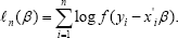
We first give a brief review of the existing method of variable selection. Assume ϵ=y-x'β has some known density f(.) (such as normal), with possibly some unknown parameter(s). For simple of discussion we assume there is no unknown parameters. Then the log-likelihood is
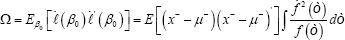
Let  be the MLE of β (when f (.) is the standard normal density, is just the least squares estimate). If we delete k(≤d) columns of Xn and the corresponding components of β denote the remaining covariate matrix as Xn- and the resulting β as β- and the corresponding MLE as -. Then under the hypothesis H0 : the deleted columns of Xn has no effects, or equivalently the deleted components of β are all zeros, then asymptotically
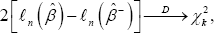
Where xk2 is the chi-squared distribution with k degrees of freedom. Let xd2(1-α) be the (1 -α)th upper quantile of the xk2 distribution, if (1-α) then H0 is rejected at significance level α, and its’ not good to delete these columns of Xn; otherwise we accept H0 and delete these columns of Xn. There are some other methods to select columns of Xn such as AIC, BIC and their variants, as in the model selection field. In These methods, the optimal deletion of columns of Xncorresponds to the best model selection, which maximize the AIC or BIC. These methods are not as solid as the above one, as may sometimes depending on eye inspection to choose the model which maximize the AIC or BIC.
All the above methods require the models under consideration be nested within each other, i.e., one is a sub-model of the other. Another more general model selection criterion is the minimum description length (MDL) criterion, a measure of complexity, developed by Kolmogorov [4], Wallace and Boulton, etc. The Kolmogorov complexity has close relationship with the entropy, it is the output of a Markov information source, normalized by the length of the output. It converges almost surely (as the length of the output goes to infinity) to the entropy of the source. Let ζ = {g(.,.)} be a finite set of candidate models under consideration, and e = {θj;j= 1,...,h.} be the set of parameters of interest. θi may or may not be nested within some other θj, or θi and θj both in È may have the same direction but with different parametrization. Next consider a fixed density f(.θj) with parameter θj running through a subset  to emphasize the index of the parameter, we denote the MLE θj of under model f(.|.) by
  (instead of by
  to emphasize the dependence on the sample size), I(θj) the Fisher information for fyj under θj (θj) its determinant, and θj the dimension ofθj Then the MDL criterion [16] chooses θj to minimize

This method does not require the models be nested, but still require select/delete some whole columns, and does not apply to our case.
Now come to our question, which is non-standard and we are not aware of a formal method to address this problem. However, we think the following question is of practical meaning. Consider deleting some of the components within fixed k(k≤d) columns of Xn the deleted proportions for these columns are γ1,......γk(0<γj<1) Denote xn-for the remaining covariate matrix, which is xn with ynβ+òn
After the partial deletion of covariates, the model becomes ynβ+òn
Note that here β and β- have the same dimension, as no covariate is completely deleted. β is the effects of the original covariates, β- is the effects of the covariates after some possible partial deletion. It is the effects of the effective covariates. Thus, though β and β- have the same structure, they have different interpretation. The problem can be formulated as testing the hypothesis:
H0:β=β- vs H1:β≠β-
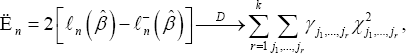
Note that different from the standard null hypothesis that some components of the parameters be zeros, the above null hypothesis is not a nested hypothesis, or -β- is not a subset of -β, so the existing Wilks’ theorem for likelihood ratio statistic does not directly apply to our problem. Denote ln-(β) be the corresponding log-likelihood based on data (ynXn-) and the corresponding MLE as -β- Since after the partial deletion, β- is the MLE of under a constrained log-likelihood, while is the MLE under the full likelihood, we have  Parallel to the log-likelihood ratio statistic for (whole) variable deletion, let, for our case,
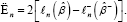
Let (j1,......jk) be the columns with partial deletions, Cjr={i:xjr,i is deleted 1ࣘiࣘn} 1 be the index set for the deleted covariates in the jrthcolumn be the cardinality of Cjr thus mar = | Ch \ jn(r = 1,...,k). We first give the following Proposition, in the simple case in which the index sets Cjr are mutually exclusive. Then in Corollary 1 we give the result in more general case in which the index sets Cjr are not need to be mutually exclusive. For given Xn, there are many different ways of partial column deletions, we may use Theorem 1 to test each of these deletions. Given a significance level a, a deletion is valid at level α if En<X2(1-α), where X(1 -α) is the (1 -α) upper quantile of the distribution, which can be computed by simulation for given γ1,......γk
The following Theorem is a generalization of the Wilks [1] Theorem. Deleting some whole columns in Xn, corresponds to γ = l (j = 1,..., k) in the theorem, and then we get the existing Wilks' Theorem.
Theorem 1
Under Ho, suppose Cjr⋂ Cjr=Δ the empty set, for all 1 ≦r≠ , then we have
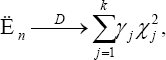
Where x12......xk2 are iid chi-squared random variable with 1-degree of freedom. The case the Cjr are not mutually exclusive is a bit more complicated. We first re-write the sets Cr such that
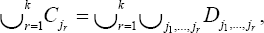
where the D r's are mutually exclusive, Dj1,....,DJk are index sets for one column of Xn only; the dju1’s are index sets common for columns j1 and j2 only; the Dj1,j2,j3’s are index sets common for columns j1 j2 and j3 only,.... Generally some of the Dj1,.....jr's
are empty sets. Let γj1,.....jr=|Dj1,.....jr| be the cardiality of Dj1,.....jr and γj1,.....jr=|Dj1,.....jr|/n(r=1,....,k). By Examining the proof of Theorem 1, we get the following corollary which gives the result in the more general case.Corollary 1: Under H0, we have
Where the x2j1,......,jr's are all independent chi-squared random variables with r-degrees of freedom (r=1,.....,k)
Below we give two examples to illustrate the usage of Proposition.
Example 1: n = l000, d = 5 k = 3. Columns (1,2,4) has some partial deletions with C1 = {201,202,....,299,300}, C2 ={351,352,...,549,550}, C3 = {601,602,...,849,850} the have no Cj's overlap; γ1 = 1 / 10 γ2 = 1/5, γ3 = 1/4. o by the Proposition, under Ho we have
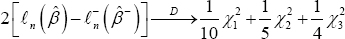
Where all the chi-squared random variables are independent, each has 1 degree of freedom.
Example 2: n = 1000 , d = 5, k = 3 Columns (1,2,4) has some partial deletions with c1 ={101,102,...., 299,300;65i, 652, ...,749,750},
C2 = {201,202,...,349,350},
C3 = {251,252,..., 299,300; 701,702,799,800}. In this case the Cj’s have overlaps, the Proposition can not be used directly, so we use the Corollary. Then A = {101,102,...,199,200}, D2 = {301,302,...,349,350}, D3 ={701,702,...,799,800},
D1,2,3 = {201,202,...,249,250}, D1,3 = {701,702,...,749,750}
D1,2,3 ={251,252,...,299,300}, γ1 = 1/5 γ2 = 1/20, γ3 = 1/10, γ1,2 = 1/20, y,3 = 1/20, γ2,3 = 0, γw = 1/20. So by the Corollary, under H0 we have

where all the chi-squared random variables are independent, with X12 x22 and X32 are each of 1 degree of freedom, x1,22 and X,1,32 are each of 2-degrees of freedom, and x1,22 and X,1,32 is of 3-degrees of freedom. Next, we discuss the consistency of estimation of - under the null hypothesis Ho Let x = xr with probability
Theorem 2
Under conditions of Theorem 1,
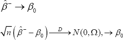
Where,
To extend the results of Theorem 2 to the general case, we need the following more notations. Let x(j1,....,jk) be an i.i.d. copy of data in the set Dj1,.....,jk. Let x-=x-j1,.....,jk with probability γ j1,.....,jk(r=0,1,....,k) where x-j1,.....,jk is an i.i.d. copy of the j1,.....,jk's, whose components with index in Ch
Corollary 2: Under conditions of Corollary 1, results of Theorem 2 hold with x given above.
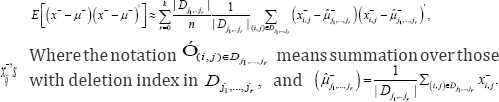
Computationally E[(x--μ-)(x--μ-) is well approximated by
Simulation study and application
Simulation study : We illustrate the proposed method with two examples, Example 3 and Example 4 below. The former rejects the null hypothesis H0 while the latter accepts. In each case we simulate n=1000 i.d. data with response yi and with covariates xi=(xi1,xi2,xi3,xi4,xi5) We first generate the covariates, sample the xi’s from the 5-dimensional normal distribution with mean vector μ= (3.1,1.8,-0.5,0.7,1.5)' and a given covariance matrix Ã. Then we generate the response data, which, given the covariates. The are yi's, generated as = x,-β + °, (i = 1,...>"), Po =(0.42,0.11,0.65,0.83,0.72)' the òi's are i.i.d. N(0,1). Hypothesis test is conducted to examine if the partial deletion is valid or not. Significant level is set as α= 0.05. The experiment repeated 1000 times, prop represents the proportion Ė> x2(1-α).
Example 3: In this example, we are interested to know whether covariates with  can be deleted. Five data set with different β0 values are simulated. With γ=(γ1,....,γk) the results are shown in Table 1. We see that the proportion of rejecting H0 (Prop) are all smaller than in the five set of β0. This suggests that covariates with should not be deleted at 0.05 significance level. Example 4. In this example, the original X as in Example 3, but now we replace the entries in first 100 rows and first three columns by ò, where òN(0,1/9) We are interested to see in this case whether these noises can be deleted, i.e. H0 can be rejected or not. The results are shown in the following. We see that the proportion of rejecting H0 (prop) are all greater than 0.95 for the five sets of β0. It suggests that the data provided strong evidence to conclude that the deleted value are noises and they are not necessary to the data set at 0.05 significance level.

Application to real data problem
We analyze a data set from the Deprenyl and Tocopherol Antioxidative Therapy of Parkinsonnism, which is obtained from The National Institutes of Health (NIH)[17]. It is a multicenter, placebo-controlled clinical trial that aimed to determine a treatment for early Parkinson's disease patient to prolong their time requiring levodopa therapy. The number of patients enrolled was 800. The selected object were untreated patients with Parkinson’s disease (stage I or II) for less than five years and met other eligible criteria. They were randomly assigned according to a two-by-two factorial design to one of four treatment groups:
Placebo
Active tocopherol
Active deprenyl
Active deprenyl and tocopherol.
The observation continued for 14±6 months and reevaluated every 3 months. At each visit, Unified Parkinson’s Disease Rating Scale (UPDRS) including its motor, mental and activities of daily living components were evaluated. Statistical analysis result was based on 800 subjects. The result revealed that no beneficial effect of tocopherol. Deprenyl effect was found significantly prolong the time requiring levodopa therapy which reduced the risk of disability by50 percent according to the measurement of UPDRS. Our goal is to examine whether some of the covariates can be partially deleted. The response variables to examined are PDRS, TREMOR,S/E ADL by Rater, PIGD, Days from enrollment and Days from enrollment to Need for LEVODOPA. The covariates are Age, Motor and ADL for all these responses [18]. The deleted covariates are the ones with values below the γth data quantile, with γ= 0.0 1,0.02,0.03 and 0.05. We examine the responses one by one. The results are shown in Tables 2-5 below.
In Table 3, response TREMOR is examined. For covariable Age, the likelihood ratio E, is larger than the cutoff point x2(1-α) at 0.03 and 0.05 levels, it suggests that for Age, partial deletions with these proportions are not valid. For covariable Motor, e , is smaller than the cutoff point x2(1-α) at the 0.05 and 0.1 levels, this covariable can be partially deleted at these proportions. For covariable of ADL, with deletion proportions 0.01-0.1, the likelihood ratio  is smaller than x2(1-α) which suggest that the lower percentage of 1%-10% can be deleted. In Table 4, PIGD is the response variable. For covariable age, is larger than the cutoff point <2(1 -α) at 0.01, 0.02, 0.03 and 0.05 level, suggests that it cannot be partially deleted with these proportions [19]. For covariable Motor, dan is smaller than cutoff point x2(1-α)up>at the deletion proportions of 0.02 and 0.03, suggests that the lower percentage of 2% and 3% can be deleted from the covariable Motor. For the variable ADL,E, is larger than the cutoff point Q (1-α) at the delete proportion of 0.01, 0.02, 0.03 and 0.05, hence partial deletion is not valid.
In Tables 5, the response is PDRS. The likelihood ratios En of Age, Motor and ADL all are larger than x2 (1 -α) at the
deletion proportions of 0.01, 0.02, 0.03 and 0.05. Thus the null hypothesis are rejected at all these proportions. Note that the coefficient for Age is insignificant, and hence the corresponding En values with deleted proportions are senseless Appendix.


Concluding remarks
We proposed a method for partial variable deletion, which is a generalization of the existing variable selection. The question is motivated from practical problems. It can used to find the effective ranges of the covariates, or to remove possible noises in the covariates, and thus the corresponding estimated effects are more interpretable. The procedure is a generalization of the Wilks likelihood ratio statistic, and is simple to use. Simulation studies are conducted to evaluate the performance of the method, and it is applied to analyze a real Parkinson disease data as illustration.
References
- Wilks SS (1938) The large-sample distribution of the likelihood ratio for testing composite hypotheses. Annals of Mathematical Statistics 9: 6062.
- Akaike H (1974) A new look at the statistical identification model. IEEE Transaction on Automatic Control 19: 716-723.
- Schwarz G (1978) Estimating the dimension of a model. Annals of Statistics 6: 461-464.
- Kolmogorov A (1963) On tables of random numbers. Sankhya Ser A 25: 369-375.
- Hansen M, Yu B (2001) Model selection and the principle of minimum description length. Journal of American Statistical Association 96: 746774.
- May RJ, Maier HR, Dandy GC, Fernando TG (2008) Non-linear variable selection for artificial neural networks using partial mutual information. Environmental Modelling and Software 23: 1312-1326.
- Mehmood T, Liland KH, Snipen L, Saeb S (2012) A review of variable selection methods in partial least squares regression. Chemometrics and Intelligent Laboratory Systems 118: 62-69.
- Wang L, Liu X, Linag H, Carroll R (2011) Estimation and variable selection for generalized additive partial linear models. Annals of Statistics 39: 1827-1851.
- Liu X, Wang L, Liang H (2011) Estimation and variable selection for semiparametric additive partial linear models. Stat Sin 21(3): 12251248.
- Tibshirani R (1996) Regression shrinkage and selection via the lasso. Journal of the Royal Statistical Society B 58: 267-288.
- Tibshirani R (1997) The lasso method for variable selection in the Cox model. Stat Med 16(4): 385-395.
- Fan J, Li R (2001) Variable selection via non-concave penalized likelihood and its oracle properties. Journal of the American Statistical Association 96: 1348-1360.
- Fan J, Li R (2002) Variable selection for Cox's proportional hazards model and frailty model. Annals of Statistics 96: 1348-1360.
- Wang HX, Leineweber C, Kirkeeide R, Svane B, Theorell T, et al. (2007) Psychosocial stress and atherosclerosis: family and work stress accelerate progression of coronary disease in women. The Stockholm Female Coronary Angiography Study J Intern Med (3): 245-254.
- Shara NM, Wang H, Valaitis E, Pehlivanova M, Carter EA, et al. (2011) Comparison of estimated glomerular filtration rates and albuminuria in predicting risk of coronary heart disease in a population with high prevalence of diabetes mellitus and renal disease. Am J Cardiol 107(3): 399-405.
- Rissanen J (1996) Fisher information and stochastic complexity. IEEE Transactions on Information Theory 42: 40-47.
- Bickel PJ, Klaassen CA, Ritov Y, Wellner JA (1993) Efficient and Adaptive Estimation for Semiparametric Models, Johns Hopkins University Press, Baltimore, Maryland, USA.
- Shoulson I (1989) Deprenyl and tocopherol antioxidative therapy of parkinsonism (DATATOP). Parkinson Study Group. Acta Neurol Scand Suppl 126: 171-175.
- http://www2.math.umd.edu/slud/s701/WilksThm.pdf


