


Bayes Estimation under a Finite Mixture of Truncated Generalized Cauchy Distributions Based On Censored Data with Application
Saieed F Ateya1,2* and Hesah A Al Khald1
1Department of Mathematics & Statistics, Taif University, Saudi Arabia
2DDepartment of Mathematics, Assiut University, Egypt
Submission: December 04, 2017; Published: February 19, 2018
*Corresponding author: Saieed F Ateya, Department of Mathematics & Statistics, Taif University, Saudi Arabia, Tel: 9.66545E+11; Email: ca.uzuke@unizik.edu.ng
How to cite this article: Saieed F A, Hesah A Al Khald. Bayes Estimation under a Finite Mixture of Truncated Generalized Cauchy Distributions Based On Censored Data with Application. Biostat Biometrics Open Acc J. 2018; 5(1): 555652. DOI: 10.19080/BBOAJ.2018.05.555652
Abstract
In this paper, the Bayes estimates (BE's) of the parameters, reliability and hazard rate functions of a finite mixture of truncated generalized Cauchy distributions are obtained based on type-I, type-II and progressively type-II censored samples. A simulation study is carried out to study the behaviour of the mean squared errors (MSE's) of the estimates. All previous parameters and functions are obtained based on generated type-I, type-II and progressively type-II censored samples generated from a real data set as illustrative application.
Keywords: Truncated generalized Cauchy distribution; Bayes estimation; MCMC algorithm; Finite mixture models; Type-I censoring; Type-II censoring; Progressively type-II censoring
Abbreviations: BE's: Bayes Estimates; MSE's: Mean Squared Errors; TGCD: Truncated Generalized Cauchy Distribution; PDF: Probability Density; CDF: Cumulative Distribution Function; SF: Survival Function; HRF: Hazard Rate Function; LF: Likelihood Function
Introduction
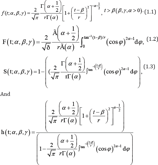
The Cauchy distribution is a symmetric distribution with bell shaped density function as the normal distribution but with a greater probability mass in the tails. The distribution is often used in the cases which arise in outlier analysis. The Cauchy distribution has received applications in many areas, including biological analysis, clinical trials, stochastic modelling of decreasing failure rate life components, queuing theory, and reliability. For data from these areas, there is no reason to believe that empirical moments of any order should be infinite. Thus, the choice of the Cauchy distribution as a model is unrealistic since its moments of all orders are not infinite. The introduced truncated generalized Cauchy distribution (TGCD) can be a more appropriate model for the kind of data mentioned. For more details about Cauchy and truncated generalized Cauchy distributions, see the book by Johnson et al. [1] which covers the Cauchy distribution in many of its aspects starting from the history, properties, developments and applications up to the most recent research done in the subject matter, to the date of the book's publication. Also see, Ateya & AL-Hussaini [2] and Ahsanullah [3] which studied the TGCD extensively The probability density (PDF), cumulative distribution function (CDF), survival function (SF) and hazard rate function (HRF) of the TGCD with parameters (a,p,y) are given, respectively, by
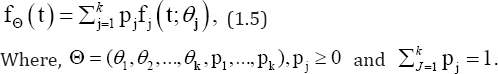
The mixture models are very important in the theoretical and applied fields especially in case of the heterogeneous population. For details about mixture models, see McLachlan & Peel [4], Titterington, Smith & Makov [5], Bozidar et al. [6] and Satheesh & Manju [7]. A random variable T is said to have a finite mixture of TGCD's with parameters θ=(αj,βj,γj),j=1,2,....,k, if its pdf is given by
The corresponding CDF, SF and HRF are given by

Where, fj(t;θj),Fj(t;θj) and Sj (t;θj) can be obtained from equations (1.1)-(1.3) after replacing θ=(α,β,γ)by θj(αj,βj,γj).
Prior analysis and some important algorithms
In this section, a suggested prior and some important algorithms will be introduced.
Prior analysis: Suppose that the prior belief of the experimenter is measured by a prior PDF π(p,α12,γ1γ2,β)constructed as follows:
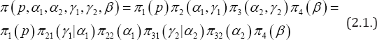
Suppose that π1(p) is Beta (c1,c2),π21(γ1/α1),is Gamma (c3,β1),π22(α1)is Gamma (c4,c5),π31(γ2/α2) is Gamma (c4,c5),π32(γ2/α2)is Gamma(c7,c8 and finally π4(β) is Gamma(c9,c10with respective densities
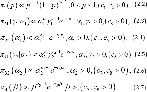
From equations (2.2) to (7.7) in equation (2.1), we can write the prior PDF of the parameters (p,α12,γ1γ2,β)as follows:
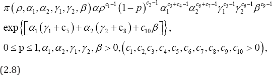
Where, (c1,c2,c3,c4,c5,c6,c7,c8,c9, and are the prior parameters.
Gibbs sampler
Gibbs Sampler is a method used to generate a random sample θ1,θ2,....,θmfrom the posterior PDF π(θ/t) as follows:
Let θ0=(è01,....,è0k) be an initial values [may be actual values of parameters, or may be the estimated values using any method]
2- Generate θ11 from π*(θ1/θ02,θ03,....,θ0k,t).
3- Generate θ11 from π*(θ2/θ11,θ03,....,θ0k,t).
4- Generate θ11 from π*(θi/θ11,θ12,....,θ1k-1, θ0i+1,....,θ0k,t).
5- Generate θ1k from so we generate π*(θk/θ11,θ12,....,θ1k-1,t) θ1,=θ11,....,θ1k)
6- Repeat steps 1-5 m times we get θ1,θ2,....,θm
Metropolis-Hastings algorithm
Is a method used to generate a number θji from the posterior PDF π*(θi/θj1,θj2,....,θji-1, θj-1i+1,....,θj-1k,x)This method can be summarized in the following steps:
1- Generate θ*ifrom a suitable PDF f(θ)
A- *min{1,A},
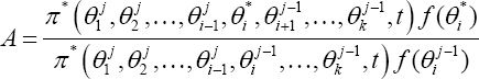
3- Generateu from μ(0,1)
4- If ,A<U then accept θ*i as θ*iJ, else *θ*iJ-1�� go to step1.
Markov chain monte carlo (MCMC) method
Let θ=(θ,θ,....,θk)be a parameters vector with a posterior PDF π*(θ\t), t=(t1,t2,....,tn)the vector of observations. If θ1,θ2,....,θm where θi=(θi1,θi is a random sample of size m generated from ()*|,t�� then the BE of a function θ(θ1) based on squared error (SE) loss functions is given by
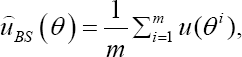
To generate from the posterior PDF π*(θ/t) we will use Gibbs sampler and Metropolis.Hastings techniques. For more details about the MCMC method, see, for example Jaheen & Al-Harbi [8], Press[9], Upadhyaya et al. [10] and Upadhyaya & Gupta[11]
Bayes estimation
In this section, the BE's of all parameters, survival and hazard rate functions will be estimated based on type-I, type-II and progressive type-II censoring schemes.
Bayes Estimation Based on type-I censoring scheme
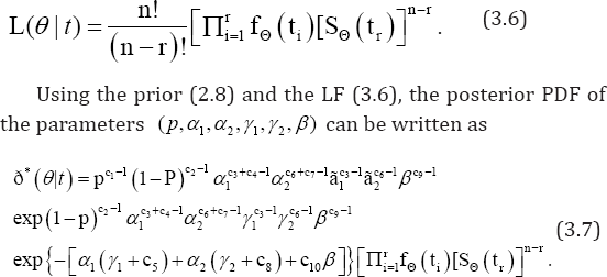
Suppose that we have n items from a finite mixture TGCD's, with equal location parameters (P = P2 = P). All items are put on a life testing experiment. Suppose that r units have failed during the interval (0,t0) and (n-r) units are still active, where t0 is a predetermined time. Let t1,..,tn be a random sample from the mixed population. The exact lifetime of an item will be observed only if t, < t0, i = i,2,...,n. This is known as type-I censored sample. The likelihood function(LF) based on type-I censored sample, see Lawless[12], may be written as
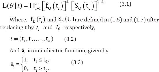
Using the LF (3.1) and the prior (2.8), the posterior PDF of the parameters (p,α1,α2,γ1,γ2,β) can be written as
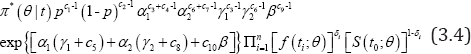
To estimate the parameters and functions p,α1,α2γ1,γ2,β survival and hazard rate functions at time t, we define a function u(p,α1,α2,γ1,γ2,β) as
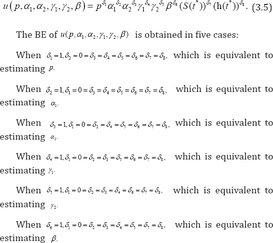
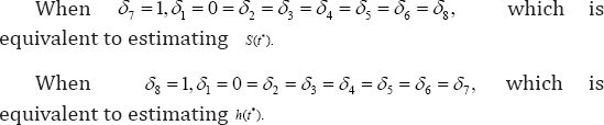
Then, MCMC algorithm will be used to estimate all mentioned parameters and functions
Bayes estimation based on type-II censoring scheme
Assume that we put items from a finite mixture of TGCD's in a life testing experiment. Instead of continuing until all n items have failed, the experiment is terminated at the time of the r* item failure. Such test can save time and money, since it could take a very long time for all items to fail. Suppose that ti
 and the same is done as 3.1.
Bayes estimation based on progressively type-II censoring scheme
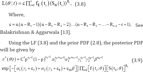
The progressive type-II censored model is of importance in the field of reliability and life testing. Suppose nidentical units are placed on a lifetime test. At the time of the ith failure, Ri surviving units are randomly withdrawn from the experiment,1 < i < r. Thus, if r failures are observed then R, + R2 +...+Rr, units are progressively censored, hence n = r+r, + r2 + ...+Rr and T,Mn < TMrn <...< TMr" describe the progressively censored failure times, where M = ( r,, R,..., Rr ) and E1r=,Ri = n - r. The likelihood function based on progressively type-II censored data t = (tMrn,t(2;r:n),o o ?,C») which can be written for simplicity as t = (t,, t2,..., tr ) is given by
 and the same is done as 3.1.
Where,
C* = n(n-Rj-1)(n-Rj -R2-1)....(n-Rj -R2 -...-Rrf -r-1), and also the same is done as 3.1 and 3.2
Simulation study and data analysis
In this section, all studied parameters and functions will be estimated based on type-I, type-II and progressive type-II censoring samples from generated and real data.
Simulation study
In this section, a simulation study is carried out to study the behavior of the MSE's. In case of j = 2, we can write p1 = p, p2 = 1 - p, then the vector of all parameters will be in the form
θ = (α1,α 2β,γ1γ2,p)
For different values of ^o and r, follow the following steps: Making use of the set of hyper parameters, the vector of the population parameters will be generated.
Making use of the generated vector of parameters θ = (α1,α2,β,γ1,γ2,p) samples of different sizes n (10, 20, 30) are generated from a mixture of two TGCD as follows:
• Generate U1 and U2 from the uniform distribution U(0,1).
• If u1 < p, generate from F1 (t;α1β,γ1) using μ2 otherwise generate from F2 (\;α2,ß,γ2) using u2.
For a value t0, we consider all values of the random variable T which are less than or equal MSE0)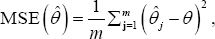 (type-I censored sample). m
Based on this sample and for different values of to> we can use the Bayes method to obtain the estimate of the vector of parameters 0. survival and hazard rate functions.
Based on the sample t1 < t2 <.. .< tr which is a type- II censored sample, we can use Bayes method, as done in case of type-I censoring, to obtain the BE's of the same vector of parameters and functions, for different values of r.
For different schemes, progressive type-II will be generated and the same is done based on the generated progressively type-II censored samples.
Repeat steps 1-6 (m) times for different samples.
The MSE's of θ over the m samples is given by:
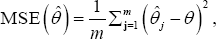
Where θ is the actual value of the vector of parameters qj and is the estimate of the vector of parameters over the sample j
In Tables 1-6 the BE's of all parameters and functions have been obtained based on Type-I, Type-II and progressively Type-II censored samples.


Data analysis
In this section, a mixture of two real data sets from Ateya & Madhagi [14] is introduced. These data are [after ordering]
2.3707, 2.4282, 2.4743, 2.4858, 2.4858, 2.5088, 2.5663, 2.6239, 2.6239, 2.6814,2.762, 3.0266, 3.1187, 3.1509, 3.5905, 3.6825, 3.6825, 3.7136, 3.7373, 3.7799, 3.8322, 3.8603, 3.8981, 3.9644, 4.059, 4.1583, 4.2577, 4.2719, 4.3326, 4.3846, 4.4275, 4.4275, 4.532, 4.554, 4.5856, 4.6172, 4.6172, 4.6488, 4.7121, 4.7355, 4.807, 5.1518, 5.166, 5.1944, 5.2369, 5.6201, 5.9607, 6.5568, 7.1529, 7.644, 7.81, 7.84, 7.938, 8.0044, 8.134, 8.526, 8.82, 8.82, 9.31, 9.31, 9.506, 9.8, 10, 10.001, 10.1, 10.3, 10.9504, 11.3302, 11.3935, 11.6, 11.8394, 12.6457, 12.9286,13.1, 13.169, 13.2, 13.3246, 13.4, 13.7, 13.7914, 13.8, 14, 14, 14, 14.0177, 14.0885, 14.1, 14.1733, 14.4, 14.6, 14.6118, 15.0645,15.5, 15.5454, 15.9698, 16.1, 16.479, 16.5, 16.9, 16.9, 17.0306,17.1, 17.2, 17.3, 17.3, 17.3, 17.3, 17.4, 17.7, 17.8, 17.8793,17.9, 18.2, 18.9, 19.2357, 19.4, 20.0812, 21.5, 22.7587, 23.4,23.6, 24.1, 25, 26.4226, 26.5, 26.7, 26.7, 26.8, 26.9, 27.6, 28.4,28.9, 29.4, 29.8, 30, 30.157, 30.4, 30.9, 31.2, 31.8, 32.9, 33.9, 34.4551, 35.5, 37.6963, 37.7, 39.8, 40.5852, 41.1, 42.5, 44.6719,46.2, 48.829, 51.9, 54.3249, 55.5, 58.2, 60.3141, 62.1, 65.5281, 67.2192, 67.7, 72.4151, 76.7, 79.8316, 85.5389, 86.3, 92.0212, 94, 97.6, 99.2082, 101.3, 105.3, 106, 107.6, 107.9, 109.3, 110, 110.5, 112.8, 115.4, 118.5, 120, 120.3, 120.5, 121.9, 124.1, 126.1,131.3, 133.8, 135.4, 137.9, 139.5, 141.9, 142.8, 145.8, 146.5, 149.7, 150.6, 153.5, 158.6, 161.3, 163.9, 168.3, 174, 176.7, 180.9,184.3, 190.3, 196.8
The BE’s of the parameters, survival and hazard rate functions based on type-I, type-II and progressively type-II under the previous real data set are summarized in Tables 1-6.
In most cases, observe the following:
• For fixed and and by increasing the sample size n, we often get smaller MSE’ s.
• For fixed sample size n and by increasing the censoring values fixed t_0and r, we often get smaller MSE’ s.
• The largest values of and in each case represent the complete sample case.
• In progressively type II, for fixed n, we often get smaller MSE’ s by increasing r.
References
- Johnson NL, Kotz S, Balakrishnan N (1995) Continuous Univariate Distributions, V-2, (2nd edn) edition, Wiley, New York, USA Pg No. 784.
- Ateya SF, AL-Hussaini, EK (2012) On truncated generalized Cauchy distribution. J Math Comput Sci 2: 289-304.
- Ahsanullah M (2015) Some Inferences on Truncated Generalized Cauchy Distribution. AfrikaStatistika 10: 815-826.
- McLachlan GJ, Peel D( 2000) Finite Mixture Models. Wiley, New York, USA.
- Titterington DM, Smith AFM, Makov UE (1985) Statistical Analysis of Finite Mixture Distributions. Wiley, New York, USA.
- Bozidar VP, Gauss C, Edwin MO, Marcelino ARP (2017) A new extended mixture normal distribution. Math Commun 22: 53-73.
- Satheesh KC, Manju L (2017) A Note on Logistic Mixture Distributions. Biostat Biometrics Open Acc J 2(5): BBOAJ.MS.ID.555598.
- Jaheen ZF, Al-Harbi, MM (2011) Bayesian estimation for the exponentiated Weibull model via Markov chain Monte Carlo simulation. Communications in Statistics: Simulation and Computation 40: 532543.
- Press SJ (2003) Subjective and Objective Bayesian Statistics: Principles, Models and Applications, Wiley, New York.
- Upadhyaya SK, Vasishta N, Smith AFM (2001) Bayes inference in life testing and reliability via Markov chain Monte Carlo simulation. Sankhya A 63: 15-40.
- Upadhyaya SK, Gupta A (2010) A Bayes analysis of modified Weibull distribution via Markov chain Monte Carlo simulation. J of Statist Comput and Simul 80: 241-254.
- Lawless JF (2003) Statistical Models and Methods for Lifetime Data, (2nd edn) Wiley, New York, USA.
- Balakrishnan N, Aggarwala R (2000) Progressive Censoring: Theory, Methods, and Applications. Springer.
- Ateya SF, Elham A Madhagi (2013) On multivariate truncated generalized Cauchy distribution. Statistical Papers 54: 879-897.


