


Impact of Raising Copayment and/or Reducing Reimbursement Benefits on Healthcare according to "Disequilibrium Bivariate Distribution"
Shanmugam R*
Honorary Professor of International Studies, School of Health Administration, Texas State University, USA
Submission: November 23, 2017; Published: February 15, 2018
*Corresponding author: Ramalingam Shanmugam, Honorary Professor of International Studies, School of Health Administration, Texas State University, San Marcos, TX 78666, USA; Email: rs25@txstate.edu
How to cite this article: Shanmugam R . Impact of Raising Copayment and/or Reducing Reimbursement Benefits on Healthcare according to "Disequilibrium Bivariate Distribution". Biostat Biometrics Open Acc J. 2018; 5(1): 555651. DOI: 10.19080/BBOAJ.2018.05.555651.
Abstract
This article probes and illustrates the consequences of raising co-payment and/or reducing reimbursement benefits on healthcare operations. For this purpose, a new bivariate count model with its properties is introduced. The model is named "disequilibrium bivariate Poisson distribution”. An analytic methodology and healthcare management implications are devised to perform data analysis by the healthcare managers. The Australian Health Survey of year 1977-1978 data are considered in the illustration. Thoughts for further research direction are suggested.
Keywords: Size-biased Poisson sampling; Regression; Survival function; chi-squared distribution
Abbreviations: GDP: Gross Domestic Product; MLE: Maximum Likelihood Estimator; DBPD: Disequilibrium Bivariate Poisson Distribution
Motivation
Healthcare is a significant part of every country's economy. In 2011, the healthcare industry consumed about 9.3 percent of the US gross domestic product (GDP), 10 percent of the Canada’s GDP, and 11 percent of the France's as well as in Germany’s GDP. Based on a random sample of 337 sex offenders, who received treatment in the Ontario region, Canada, during the years 1993 to 1998, Mailloux et al. [1] reported an increase of risk to die due to over-prescription. Ding et al. [2] stated that China's health reforms in 2009 resulted in significant changes in the prescribing patterns. He [3] warned that over-prescription increased the threats of malpractice/litigation lawsuits. Sacarny et al. [4] announced that over-prescribing threatened Medicare benefits. Based on a study examining 230,800 prescriptions written during the period 2007 and 2009 in 784 community hospitals over 28 cities across China, Parveen et al. [5] mentioned that over-prescribing caused incorrect, ineffective and insecure treatment, exacerbation or continuation of illness, and increased the healthcare cost. Li et al. [6] proved the existence of a substantial overprescribing against the recommendation by the World Health Organization. The German’s healthcare reform of the year 1997 resulted in a significant reduction of the number of visits by the patients [7,8]. They wondered whether the extra reimbursement possibility from the insurance coverage induce the physicians to write more prescriptions? In December 2011, the Centers for Medicare and Medicaid Services announced that about 30% of the healthcare spending is waste. According to an administrator, the first cause for the waste was identified to be over-prescription/overtreatment of the patients. To minimize the waste, would raising the copayment and/or reducing the reimbursement benefits help? The tendencies for overprescription and frequent visit to physician is the central theme of this article.
Paradoxically, discussions concentrate on minimizing healthcare cost rather than building up healthy population and/or quality healthcare. An ancient recommendation is that an ounce of prevention is worth tons of treatments. This article hypothetically probes the impacts of raising co-payment and/or reducing reimbursement benefits in the healthcare operations. Logically, would rising of the copayment restrict the patient’s visits to physician less often than needed. Let 0≤ξ≤ 1 be the impact level of raising copayment on patient’s visitation rate, λ> 0 to the physician. Would reducing reimbursement benefits slow down physician's prescription rate. Let 0≤Ø≤1 be the impact level of reducing the reimbursement benefits on the physician’s prescription rate, θ>0. These two restrictions likely to cause disequilibrium in the chance meachanism governing the healthcare operations. This article is a pioneering attempt to formally defineand critically examine the impact of both the raising copayment onpatient's visit and the reduction of reimbursement benefits with respect to the physician's prescription. For this purpose, an appropriate new model is introduced with its properties. The model is named a disequilibrium bivariate Poisson distribution (DBPD). A data analytic methodology is devised, based on DBPD. Healthcare managers of a hospital/clinic operation and/or health insurance organization could emulate the illustration of the methodology in their pursuits.
The article is organized as follows to understand the reality for formulating strategic policies to adapt for better healthcare management. In Section 2, we derive the disequilibrium bivariate Poisson distribution and its statistical properties. We formulate a hypothesis testing procedure to check whether the impact levels. In Section3, the concepts and all derived algebraic expressions are illustrated and interpreted, using the Australian Health Study data for 1977-1978. Finally, in Section 4, a few conclusive comments and suggestions for future research direction to attain an efficient healthcare management are stated.
Derivation of "Disequilibrium Bivariate Poisson Distribution” and its properties
First, let us recognize that the healthcare practices and management do have chance oriented mechanism to deal with. The patient’s visitation and physicians prescription rates are examples and they play a vital role to improve healthcare operations. To be specific, let λ> 0 andθ> 0 denote the patient's visitation rate and the physician’s prescription rate respectively. Ifthe copayment is raised,how would it impact the visitation rate? Let it's impact level be 0≤ξ≤1. Likewise, if a reduction of reimbursement benefits is implemented, what might be it's impact level on the prescription rate? Let its impact be o <$< i. The healthcare's chance mechanism is a mix of three scenarios.
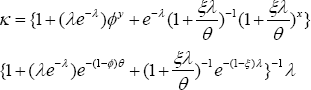
First, the scenario 1 is one in which the number,Y of precriptions exceeds the number, x of visits. Bothx and Y are random variables. Assume that the odds for the wavering patient (due to raised copayment) to make a visit is ξ/θ, because the prescription rate deflates it (Figure 1). When ξ→ o, the odds of making a visit is zero, and the scenario is void. The joint probability mass for visits and prescriptions is proportional to with an observable space, The notation , if Secondly, the scenario 2 is one in which the number, of patient's visits exceeds the number, of the precriptions. The odds for the hesitating physician (due to reduction in reimbursement benefits) to write a prescription is because the patient's visitation rate deflates it (Figure 2). When the odds of writing a prescription by a physician is zero, and the scenario-2 is void. The joint probability mass for x visits andy prescriptions is proportional to  in observable space, x = 0,1,2,...,y-i;y = 1,2,..,». The notation

Secondly, the scenario 2 is one in which the number, X of patient's visits exceeds the number ,Y of the precriptions. The odds for the hesitating physician (due to reduction in reimbursement benefits) to write a prescription  is because the patient’s visitation rate deflates it (Figure 2). When 0, the odds of writing a prescription by a physician is zero, and the scenario-2 is void. The joint probability mass for X visits and y prescriptions is proportional to in observable space,y= 0,1,2,...,x-1;x=1,2,.,».=. The notation

Thirdly, the scenario 3 is one in which the number, X of patient’s visits match the number, Y of physician’s precriptions. Raising copayment and reducing reimbursement benefits have no impact. Thejoint odds of patient’s visiting and physician’s writing prescription X9 is because of the absences of patient's wavering and the physician’s hesitaion (Figure 3). The joint probability mass for X visits y and prescriptions is proportional To  for observable space, y = 0,1,2,..., <»; x = 0,1,2,.., <».

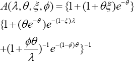
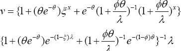
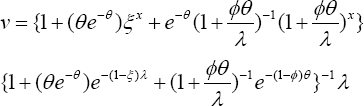
Because the three scenarios are mutually exclusive and exhaustive, the joint probability mass function for the entire healthcare chance mechansim is
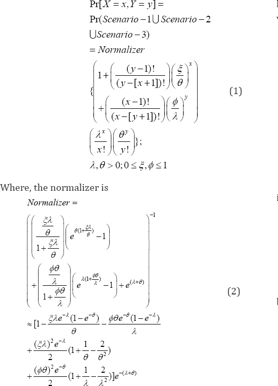
The bivariate distribution in (1) and (2) is named a �disequilibrium bivariate Poisson distribution (DBPD)�. The DBPD is a new addition to the book of several bivariate distributions, and it is helpful to analyze and interpret healthcare data as done in this article. The random variables and are dependent. See Shanmugam & Chattamvelli [9] for various for various ways of checking the independence among random variables. Shanmugam [10] presented a history of Poisson model in the healthcare data analysis. Shanmugam [11] provided a list of bivariate Poisson models. Shanmugam [12] demonstrated on how to extract data informatics to address the fear to report rapes. Shanmugam [13] constructed methodologies on how the queuing concepts helped to effectively manage the hospitals when the patients are impatient. Shanmugam [14] probed the non-adherence to prescribed medicines by patients with a bivariate model and its information nucleus. Shanmugam [15] derived a "bivariate model" for infrastructures among women with operative, natural, and no menopauses. Shanmugam [16] derived a bivariate model to identify "honesty" versus "cheating" in economic surveys to illustrate the existence of xenophobia.
One wonders about the disequilibrium level, n between the impact levels £ of raising copayment and $ of reducing reimbursement benefits. Note $ = n£, where n < 1,n = 1,n > 1, dependingrespectively on an existence of tilt to more patient's wavering to visit,perfectequilibrium, or to more physician's hesitation to write prescription. Note that the proportion not visiting a physician and nor receiving a prescription is
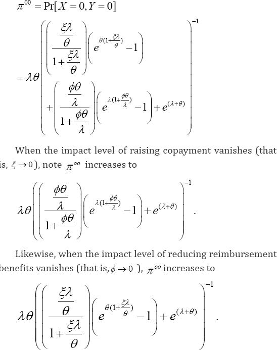
Only when both impact levels vanish (that is,ξ→0,ø→0,) π»),attains its maximum () λ øe-(λ +ø)It emphasizes that both (raising copayment and reducing reimburse benefits) are important factors to influence the proportion visiting or receiving prescriptions, which are 1-λ øe-(λ +ø) On the contrary, under complete impact levels (that is ξ→0,ø→0,) π»)decreases to 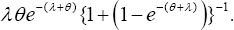
Remember that some patients might seek refill without even visiting the physician. One wonders what proportion of the patients do not visit the physician (including those do get and do not get prescriptions) and it is
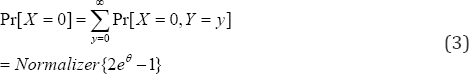
The proportion of patients making just one visit to the physician (under raised copayment) is 0Pr[1]Pr[1,]{[1(1)]}.

The jump rate (that is,  of the visitation by patients is
  using (3) and (4), which is freeø of the impact level due to reducing reimbursement benefits to the physician (Figure 4). In a situation with extremely large prescription rate (that is,ø→») the jump rate inflated visits
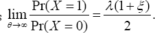

Likewise, the proportion of physicians do not write a prescription for patients visiting and not visiting is
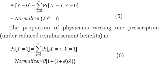
The jump rate (which is Pr(Y = 0) ) of the prescription by the physician is #{1 +$+ e){1 + (1 - e)}-1 , using (5) and (6), which is free of impact level, ç of raising copayment. In a situation
with extremely large visitation rate (that is, A — » ), the jump rate for the prescription by the physician converges to inflated prescriptions 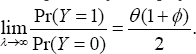
Now, let us look at the marginal stochastic trend (that is, ) of the patient's visits. Note that
The marginal probability mass function (7) of the number of visits under the raised copayment is a size biased Poisson distribution. The size bias is 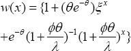
When the sampling process does not represent the intended but a different population, it is recognized as length biased. Shanmugam [17] demonstrated the effectiveness of the sample size in length biased data. Shanmugam [18] constructed a goodness-of-fit test for length-biased data with discussions on its prevalence, sensitivity, and specificity. Shanmugam [19] derived a significance testing procedure for size-biased income data. Shanmugam & Singh [20] derived an urgency biased beta distribution (which is a length-biased version) with application in drinking water data analysis. The marginal expected number of visits to physician is
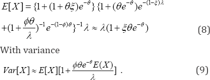
When the prescription rate becomes infinitely large (that is, 0 — »), the size bias attains the baseline value one and the stochastic pattern of the visits by the patients is Pr>[X = ] = e~AAx !. In the absence of size-bias (that is,»(?) = 0 under a convergence 0 — »), the mean in (8) approaches /I and the variance in (9) is var[X]=e[x]. It means the mean number of visits in (8) increased by an amount
 and the volatility (it is variance) changes by amount
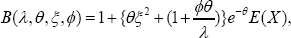 A because of the size-bias. One
also wonders whether patients would make lesser visits. For this purpose, we define lesser visits using the mode of the size-biased marginal distribution in (7). In a size-biased healthcare chance mechanism, the mode of its stochastic pattern occurs at the greatest least integer of its parameter. The cumulative Poisson purpose, we define lesser visits using the mode of the size-biased marginal distribution in (7). In a size-biased healthcare chance mechanism, the mode of its stochastic pattern occurs at the greatest least integer of its parameter. The cumulative Poisson probability is cumulative chi-squared probability. that is
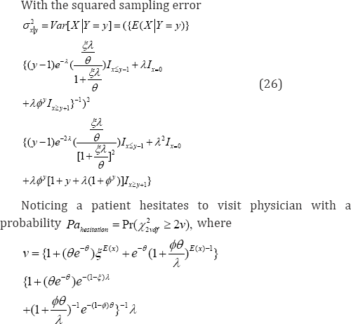
Theorem 1: A patient hesitates to visit physician, if s/he makes lesser than the most probable number
of the Poisson distribution with a probability Pa,hesitation=pr(x22vdfࣙ2v). using the relationship between the cumulative Poisson distribution and the chi-squared probability, where [] and df denote the greatest least integer and the degrees of freedom respectively.
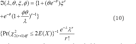
The intensity rate of the patient�fs visit to the physician in this size-biased marginal distribution (7) is then 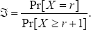
Using the link between cumulative Poisson and cumulative chi-squared distribution, the intensity rate is quantified as
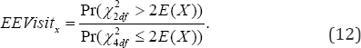
In this situation, for a given threshold t > 0 number of visits to a physician, the expected excessive visit to physician ( EEVisitx ) by a patient in (11) is
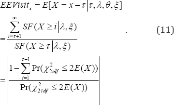
In particular with the threshold t = 2 number of visits to a physician in (11), the expected excessive visit to physician ( EEVisitx) by a patient is
The conditional probability mass function (14) of the physician�fs prescription is then
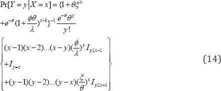
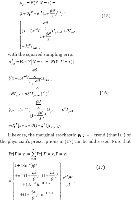
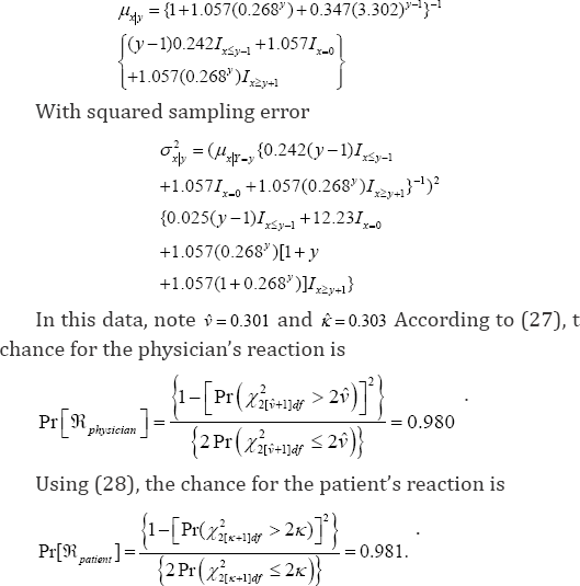
Where the indicator function 1cI=if the conditionc is true and 0cI=if the conditionc is not true. Consequently, the regression equation,[]yxEYXx��== (15) to project the number of prescriptions to be written by a physician for a given number Xx=of visits made by a patient is
The marginal probability mass function (17) of the number of prescriptions under the reduced reimbursement benefits is also a size biased Poisson distribution. The size
bias is 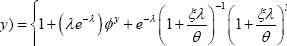 The marginal expected number (18) of prescriptions is
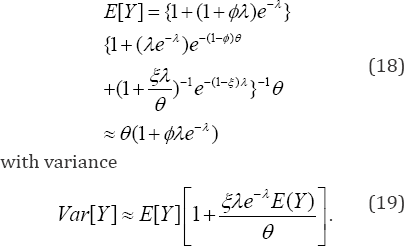
When the visitation rate by the patients becomes infinitely large (that is, A μ x), the size bias becomes the baseline value one and the stochastic pattern of the prescriptions by the physicians is Pr[Y = y] = e~e9y / y!. In the absence of size-bias (that is, w( y) = 0 under a convergence A ^ x), the mean in (18) 0 approaches and the variance in (19) is Var[Y ] = E[Y ]. It means the mean number of prescriptions in (18) increased by an amount
and the volatility changes by an amount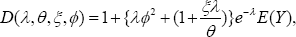 because of the size-bias.
Would physicians write lesser prescriptions? For this purpose, we define lesser prescriptions using the mode of the size-biased marginal distribution in (17). In a size-based healthcare chance mechanism, the mode of the pattern occurs at the greatest least integer of its parameter. The cumulative Poisson probability is linked to chi-squared cumulative probability for easy computations. Hence,
Theorem 2: A physician hesitates to prescribe, if s/he makes lesser than the most probable number
of the Poisson distribution with a probability ph hesitation= pr(x22kdfdࣙ2k),using the relationship betweenthe cumulative Poisson distribution and the chi-squared probability, where [] and df denote the greatest least integer and the degrees of freedom respectively.
The intensity rate (20) of the physician to prescribe with this size-biased marginal distribution (17) is then Pr[] 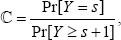 which is quantified as
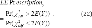
In this situation, for a given threshold0��>number of prescriptions a physician, the expected excessive prescription by the physician (EE Prescription is
EE Prescription

When the threshold2��= in (21) denoting the number of prescriptions by a physician, the expected excessive prescription (22) by a physician ()PryEEescriptionis
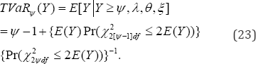
The tail value at risk (23) is for making more prescriptions beyond the threshold in the size-biased chance healthcare mechanism is
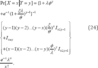
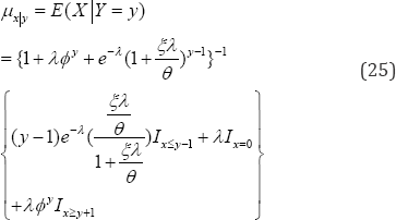
However, the conditional probability mass function (24) of the patient�fs visitation is then
When the threshold y = 2 in (21) denoting the number of prescriptions by a physician, the expected excessive prescription (22) by a physician (EE Pr escripti°ny ) is
Where, the indicator functions Ic= if the condition c is true and Ic=0if the condition is not true. Consequently, the regression equation, ==in (25) to project the number of patient�fs visitations for a given number Y=yof the prescriptions written by a physician is
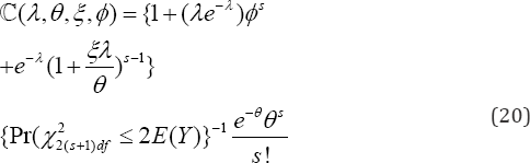
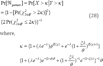
Would a physician react (that is, physician. ) to prescribe? If so, how probable such a reaction is to exist? The chance for the physician�fs reaction (27) is
connecting the four quadrants and DeMorgan�fs probability laws in the bivariate probability theory [9]. Is there reciprocity? Would the patient react (),patient. after noticing the physician hesitates to write prescriptions due to reduction of reimbursements? If so, how probable it is? The chance (28) for the patient�fs reaction is
Let us now define a parameter for the patient�s hesitation level to visit the physician, after the imposition of raising the copayment, where is as defined before. The parameter is,

Analogously, the parameter (30) captures the Physician's hesitation level to prescribe due to the reduction of reimbursements, where k is as defined in Theorem 2. That is, 30.
30.
Because Pr[ x|y = y] * Pr[ x ] and Pr[Y|X = ?] * Pr[Y ], the number of patient's visits and the number of prescriptions written by the physician are stochastically dependent. How much is then their correlation? To find it, note that
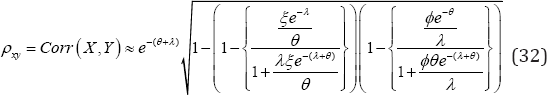
Using (31), their covariance is (,)()()(),CovXYEXYEXEY=.where ()EXand ()EYare obtained in (8) and (18) respectively. Their correlation is therefore
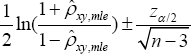
The correlation (32) depends on the impact levels of increasing copayment (that is, ��) and reducing reimbursement benefits (that is, ��). When both impact levels approach zero, their correlation,xy�� becomes zero indicating XthatY and are independent Poisson random variables. Now, we need to examine whether a sample estimate.xy�� of the correlation coefficient is significant at a specified confidence level 1(0,1)��.��. That is, the null hypothesis H0;p xyis rejected in favor of H1:p xy=0if the confidence interval .does not contain the hypothesized value zero, where ,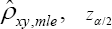 and n are respectively the maximum likelihood estimate(mle)of the correlation coefficient the standard normal percentile. The estimated correlation coefficient
 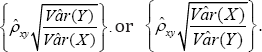 significant, which is equivalent to testing their regressioncoefficient With the mle of the parameters, note that the projected regression (33) of the number of written prescriptions by the physician [22]. (33)
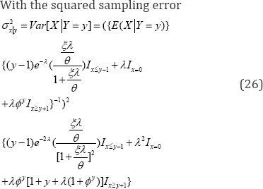
With an estimated sampling error 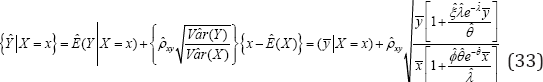 Like wise, the projected regression (34) of the number of visits made by the patients to the physician is
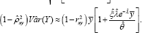
With an estimated sampling error 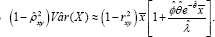
We now turn to the task of estimating the parameters A,0, — and$ of the disequilibrium bivariate Poisson distribution in (1). For this purpose, suppose a bivariate random sample (X1,y1),(x2,y2),...,(x",y<n)of sizen > 4 is drawn from the
variance xof and y, non-diagonal variance of and . Let .xyxyr��=be the sample correlation. We resort to the maximum likelihood estimator (mle) of the parameters because the mle has an invariance property. The invariance property refers that the mle of a function of the parameters is the function of their mle. Towards finding them, note that the log-likelihood function from (1) is written as
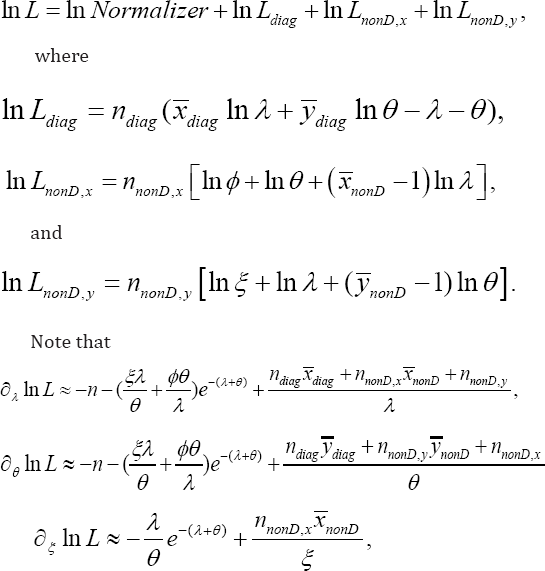
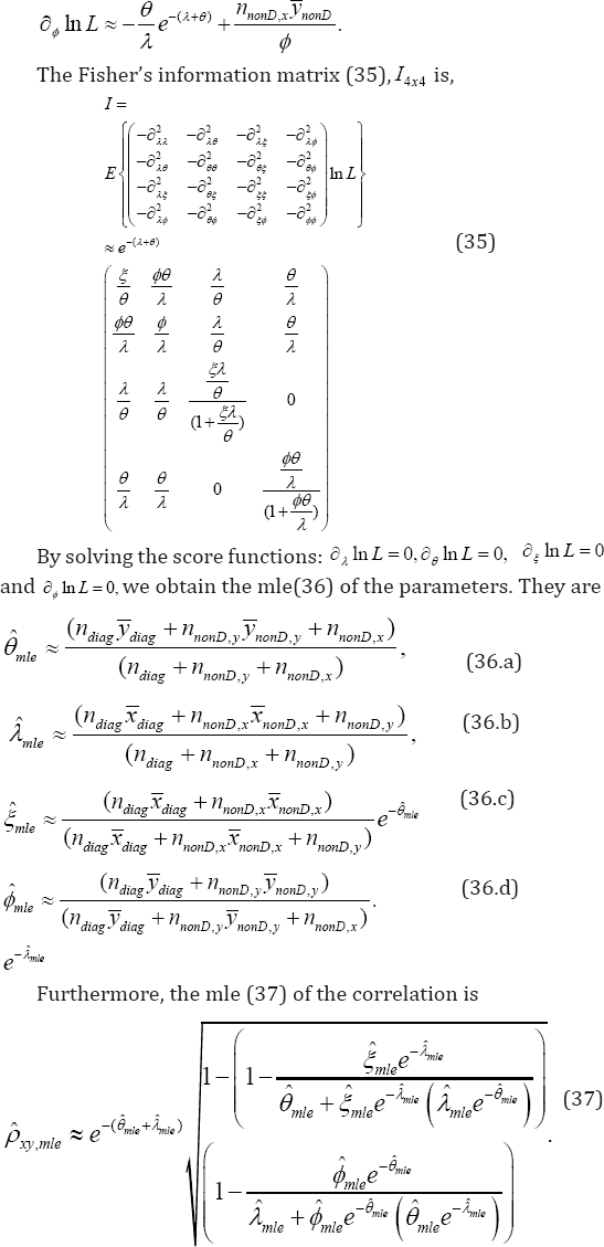
We now develop score functions based testing procedure [21] to check the validity of the hypothesis about the impact level,01�.. of raising the copayment and/or the impact level 01�..of reducing the reimbursement benefits. The score test (also known as Lagrangian multiplier test) to check the validity of a null hypothesis :0,oH�= the score statistic is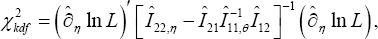 where the Fisher�s information matrix is partitioned as
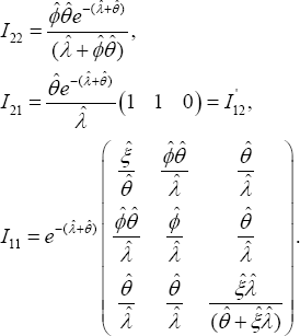
  according to the null hypothesis and the degree(s) of fre
Case 1: The null hypothesis to be tested is:0oH.= meaning the impact of raising copayment on healthcare is insignificant. The score function is 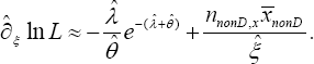
Because the degree(s) of freedom 22()krankI==1, the null hypothesis :0oH�i= is rejected with a (0,1)pvalue.. , if the statistic (38)
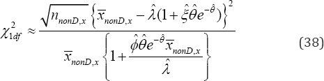
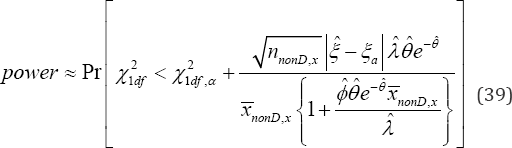
exceeds the critical value21,dfp�q . In an event the research hypothesis :aaH�i�i= is true, the statistical power (39) of accepting it is obtained and it is
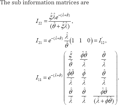
Case 2: The null hypothesis to be tested is H0:ö=0 meaning the impact of reducing reimbursement benefits on healthcare is insignificant. The score function is 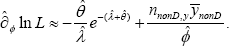 The sub information matrices are
Because the degree(s) of freedom 22()krankI==1, the null hypothesis :0oH�p=is rejected with a(0,1)pvalue.. , if the statistic in (40)
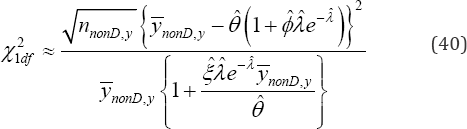
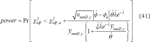
exceeds critical value 21,dfp�q.In an event the research hypothesis :aaH�p�p=is true, the statistical power(41) of accepting it is obtained and it is
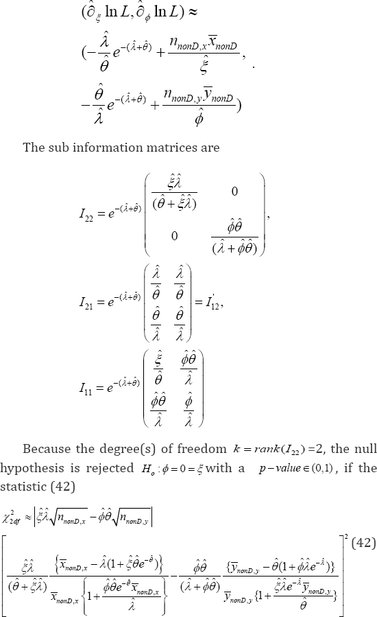
Case 3: The null hypothesis to be tested is :H0meaning that both the impact of raising copayment and reducing reimbursement benefits on healthcare are insignificant. The score vector is
In the next section, all the derived expressions are illustrated, using the Australian Health Survey data of 1977-1978.
Illustration with Australian Health Survey analysis
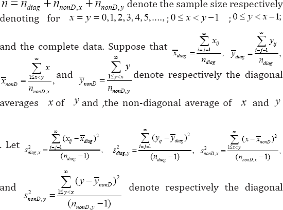
In this section, the Cameron's [23] data of n = 5,194 cases in the Australian Health Survey, in which ? = 0,l2,3,4,5 denotes the # patient's visits to the physiciany = 0,1,2,3,4,5,6,7,8 and denotes the # prescriptions written by the physicians, during 1977-1978 are displayed in Table 1. These data are analyzed and interpreted using the analytic expressions in Section 2. Note that the sample size for scenario-1 is nnonD,x = 1,125, for scenario-2 is nnonD,y = 325, and for scenario-3 is ndiag = 3,744 The correlation in (37) between the number ? of visits by the patients to the physician and the number of prescriptions written by the physicians in this survey data is p * 0.115.

The average number of visits to physician in scenario-2 is ,1.65.nonDxx= The average number of prescriptions in scenario-3 is ,1.58.nonDyy=Using (36), the parameters are estimated. The rate of visits to the physician is .0.315.mle�c. The rate of prescriptions is .1.057.mle�f. The impact level of raising the copayment on healthcare system is .0.686.mle�i.The impact level of reducing the reimbursement benefits on healthcare system is.0.268.mle�p. The odds for a wavering patient (due to raised copayment) to make a visit is
For every 10 patients who do not visit the physician, there ought to be 23 patients making a visit to the physician in spite of raising copayments. The odds for a physician(due to reduced reimbursement benefits) to write a prescription is ..8/100..�p�c�f= For every 100 physicians who do not write a prescription, there are only 8 physicians writing a prescription because of reducing reimbursement benefits.
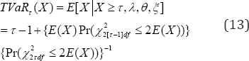
According to (8), the expected number of total visits is .()1.22EX. per annual, with an estimated variance.[]1.31VarX. using (9). According to (10), the marginal intensity rate of the patient��s visit to the physician is P 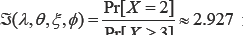 for a specified 2r=. When the threshold 2�n= number of visits to a physician, the expected excessive visit to physician by a patient in (12) is 0.849xEEVisit. with a risk (13) for making more visits beyond the threshold in the size biased chances helthcare system TVaRT(X) *3 49.. According to (15) and (16), the regression equation, Hx = E[Y|X = ?] to project the number of prescriptions to be written by a physician for a given number X = of visits made by a patient is physician, after raising the copayment, according to (29) is 8 = Pr(X126df 2 2v)/ {Pr(xL/ 2 2)}2 = 0 0178 because V = 0.301. Analogously, the physician's hesitation level to write an additional prescription, after reducing the reimbursement benefits,
According to (18) and (19), the marginal expected number of prescriptions is E(Y)* 0.346 with variance Var[Y] * 0.420 using (19). For a specified , s = 2 the intensity rate (20) of the physician to prescribe in this size-biased marginal distribution
is 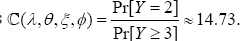 Accordingto(22)and(23),whenthe Pr[Y > 3] threshold w = 2 denoting the number of prescriptions written by a physician, the expected excessive prescription by a physician is EEPrescnpton, > 6.129 with the tail value at risk, TVaRr(X) * 3.12 for making more prescriptions beyond the threshold in the size-biased chance healthcare mechanism. The regression equation (25) to project the number of patient's visitations for a given number x = y of the prescriptions written by a physician is
The physicians and patients react in par with each other in this data. Suppose r = 4 and t = 4 are considered respectively extremely more visits to the physician and extremely more prescriptions by the physician on the annual basis. Then, the patient's hesitation to make an additional visit to the
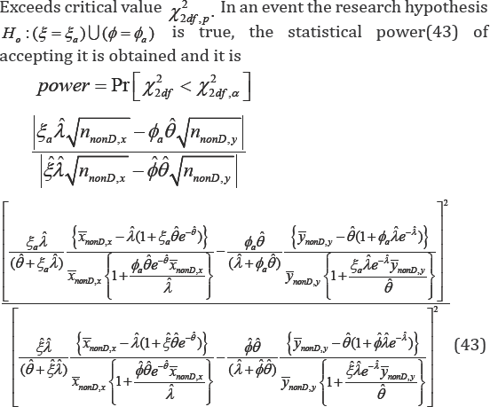
Case 3.The null hypothesis to be tested Ho 4=0 = | is meaning that both the impact of raising copayment and reducing reimbursement benefits on healthcare are insignificant in the Australian Survey data. With | * 0.68 and $ * 0.26 , the null hypothesisis rejectedHo 4 = 0 = £ is rejected with a as p -value * 0.0007, the statistic (42) x22df * 14.51. is In an event, the research hypothesis ho :(| = 0.78)U4, = 0 36)is true, the statistical power (43) of accepting it is obtained and it ispower = Pr[x22df < 5.095] * 0.921.The power curve is sketched in?
Case 1: When I = 0.68 , the null hypothesis Ho 1 = 0 (the impact of raising the copayment on the patient's visits is negligible) is rejected with a p- value * 0.0006, as the statistic xidf = 30.58. The power is the probability of accepting Ha i = i = 0.78 and it is 0.978. The power curve is sketched in Figure 5 for different values of Ia in the horizontal axis.

Case 2: With 4 = 0.268, the null hypothesis Ho 4 = 0 (the impact of reducing the reimbursement benefits on the physician's prescription is negligible) is rejected only with a p - value * 0.352, as the statistic x2f = 0.867. The power is the probability of accepting Ha 4 = ,4 = 0.36 and it is 0.951. The power curve is sketched in Figure 6 for different values of 4 in the horizontal axis.

Case 3.The null hypothesis to be tested Ho 4=0 = is meaning that both the impact of raising copayment and reducing reimbursement benefits on healthcare are insignificant in the Australian Survey data. With | * 0.68 and $ * 0.26 , the null hypothesisis rejected Ho 4 = 0 = £ is rejected with a asp - value * 0.0007, the statistic (42) x22df * 14.51. is In an event, the research hypothesis ho :(| = 0.78)U4, = 0 36)is true, the statistical power (43) of accepting it is obtained and it is power = Pr[x22df < 5.095] * 0.921.The power curve is sketched in Figure 7 for different combination values of in the x-axis $a and in the y-axis.

Comments and Conclusions
The "disequilibrium bivariate Poisson distribution" model of this article constructs probabilistic interpretation of the data evidence about the impact of hypothetical raising copayment and/or reducing reimbursement benefits in healthcare system. The significance of the estimated correlation coefficient between the number of visits made by patients and the number of prescriptions written by the physicians under this hypothetical scenario is also assessed. The chance for the patient's reaction to visit to the physician is captured, estimated and interpreted. It is worthwhile to extend this breakthrough healthcare managerial approach to discover reasons and circumstances in which the physicians lesser-prescribing tendency and/or the patients lesser visitation tendency might exist.
The healthcare managers would benefit a lot by collecting pertinent data and scrutinizing evidence data using the methodology in this article for better quality healthcare system. For the discovery to become reality, data on related covariates including the cost details, tax allowances for the prescribing physicians and the visiting patients need to be collected. The healthcare professionals ought to pay extra attention to collect such data. The analysts ought to build a multivariate regression methodology to make projections of when and how many lesser prescriptions and/or lesser visitations are possible. A discovery of reasons for such disequilibrium scenarios (quite different from an ideal situation in which one prescription per single visit of the patient occurs) is a necessity and it ought to be the future goal in this 21st century of intensive efforts to reform the healthcare practice towards cost-effectiveness and efficiencies. This article is a seminal step upward to attain such goal.
Compliance with Ethical Standards
Funding
This study was not funded by anyone. The contents are the sole opinion of the author.
Conflict of Interest
The author has no conflict of interest.
Ethical approval
No animals were involved. All applicable international, national, and/or institutional guidelines for the care and use of animals were followed.
Ethical approval
No humans were involved. All procedures performed in studies involving human participants were in accordance with the ethical standards of the institutional and/or national research committee and with the 1964 Helsinki declaration and its later amendments or comparable ethical standards.
Ethical approval
This article does not contain any studies with human participants performed by any of the authors. Informed consent was not necessary from any participant in the study because the data are secondary type from the published articles.
References
- Mailloux D, Abracen J, Serin R, Cousineau C, Malcolm B, et al. (2003) Dosage of treatment to sexual offenders: Are we overprescribing? Int J Offender Ther Comp Criminol 47(2): 171-184.
- Ding D, Pan Q, Shan L, Liu C, Gao L, et al. (2016) Prescribing patterns in outpatient clinics of township hospitals in China: A comparative study before and after the 2009 Health System Reform. Int J Environ Res Public Health, 13(7): 679.
- He AJ (2014) The physician patient relationship, defensive medicine and over prescription in Chinese public hospitals: Evidence from a cross-sectional survey in Shenzhen city. Social Science & Medicine 123: 64e71.
- Sacarny A, Yokum D, Finkelstein A, Agrawal S (2016) Medicare letters to curb overprescribing of controlled substances had no detectable effect on providers. Health Affairs 35(3): 471-479.
- Parveen Z, Gupta S, Kumar D, Hussain S (2016) Drug utilization pattern using WHO prescribing, patient care and health facility indicators in a primary and secondary health care facility. Natl J Physiol Pharm Pharmacol 6: 182-186.
- Li Y, Xu J, Wang F, Wang B, Liu L, et al. (2012) Overprescribing in China, driven by financial incentives, results in very high use of antibiotics, injections, and corticosteroids. Health Aff (Millwood) 31(5): 10751082.
- Berkhout P, Plug E (2004) A bivariate Poisson count data distribution using conditional probabilities. Statistics Neerlandica 58(3): 349-364.
- Iizuka T, Jin G (2009) The effect of prescription drug advertising on physician visits, Journal of Economics & Management Strategy 14(3): 701-727.
- Shanmugam R, Chattamvelli R (2015) Statistics for Scientists and Engineers, John Wiley Press, 111 River Street, Hoboken, NJ 070305774.
- Shanmugam R (2006) Poisson distribution, (an edited Book Chapter) in Encyclopedia of Measurement and Statistics, edited by Neil J. Salkind, Sage Press, One Thousand Oaks, California. Pp. 772-775.
- Shanmugam R (2006) Bivariate Distribution, (an edited Book Chapter) in Encyclopedia of Measurement and Statistics, edited by Neil J. Salkind, Sage Press, One Thousand Oaks, California Pp. 87-103.?
- Shanmugam R (2013) Informatics about fear to report rapes using bumped-up Poisson model. American Journal of Biostatistics. Science Publications 3(1): 17-29.
- Shanmugam R (2014) How do queuing concepts and tools help to effectively manage hospitals when the patients are impatient? A demonstration. International Journal of Research in Medical Sciences 2: 1076-1084.
- Shanmugam R (2014) Probing non-adherence to prescribed medicines? A bivariate distribution with information nucleus clarifies. American Medical Journal 5(2): 56-62.
- Shanmugam R (2014) Bivariate Distribution for infrastructures among operative, natural, and no menopauses. American Journal of Biostatistics 4: 34-44.
- Shanmugam R (2014c) A bivariate probability model to identify "honesty” versus "cheating” in economic surveys: Xenophobia is illustrated. Am J Econ Bus Admin 6: 42-48.
- Shanmugam, R. (1996). Effective sample size in length biased data. Applied Statistical Science I. In: Ahsanullah M & Bhoj, Lawrenceville, NJ, USA, pp. 89-100.
- Shanmugam R (1995) Goodness-of-fit test for length-biased data with discussion on prevalence, sensitivity and specificity of length bias, Journal of Statistical Planning and Inference 48: 277-290.
- Shanmugam R (1991) Significance testing of size bias in income data. Journal of Quantitative Economics 7: 187-294.
- Shanmugam R, Singh J (2012) Urgency biased beta distribution with application in drinking water data analysis. International Journal of Statistics and Economics 9(A12): 56-82.
- Shanmugam R (1997) Stochastic Modeling of Consumer's Diminishing Return. Journal of Italian Statistical Society 6(1): 83-92.
- Van Belle G, Fisher LD, Heagerty PJ, Lumley T (2004) Biostatistics: A methodology for the health sciences, John Wiley Press, 111 River Street, Hoboken, NJ 07030-5774.
- Cameron ACP, Trivedi FM, Piggot I (1988) A micro econometric model of the demand of health care and health insurance in Australia. Review of Economic Studies 55: 85-106.


