


Inference in Stochastic Frontier Models Based on Asymmetry
Ahmed S1, Sonia Pérez-F1, Carlos Carleos A1, Norberto C1 and Pablo Martínez C2*
1Department of Statistics and Operational Research and Mathematics Didactics, University of Oviedo, Spain
2The Dartmouth Institute for Health Policy and Clinical Practice, Geisel School of Medicine at Dartmouth, USA
Submission: September 18, 2016; Published: January 26, 2018
*Corresponding author: Pablo Martínez Camblor, The Dartmouth Institute for Health Policy and Clinical Practice, Geisel School of Medicine at Dartmouth, Hanover, NH, USA, Email: Pablo.Martinez.Camblor@Dartmouth.edu
How to cite this article: Ahmed S, Sonia P�rez-F, Carlos Carleos A, Norberto C and Pablo Mart�nez C. Inference in Stochastic Frontier Models Based on Asymmetry. Biostat Biometrics Open Acc J. 2018; 4(4): 555645. DOI: 10.19080/BBOAJ.2018.04.555645
Abstract
Stochastic frontier analysis (SFA) is often employed to study the production functions. The structure of errors is the main difference between the standard regression analysis and the stochastic frontier models; in the SFA, an independent random term with positive value is added to the usual white noise error. Conventionally, the parameters involved in the SFA are estimated and then, the convenience of using this model is tested. The authors propose to study, previously, the residuals in order to check the capacity of assuming a stochastic frontier model and then, if applicable, to estimate the parameters. With this goal, several non-parametric hypothesis testing are explored. Monte Carlo simulations suggest that, under the usual conventions, simple inference based on skewness provided competitive results and proved to be robust in the presence of outliers. Standard methods based on the maximum-likelihood obtained really poor results; they only were reasonable when both the sample size and the inefficiency term were large.
Keywords: Confidence interval; Contaminated distribution; Hypothesis testing; Stochastic frontier analysis
Abbreviations: SFA: Stochastic Frontier Analysis; MOM: Method of Moments; ML: Maximum-likelihood; WHO: World Health Organization
Introduction
The main objective of the production frontier or Stochastic Frontier Analysis (SFA) is the study of the production function. In spite of the study of the empirical estimation of production functions have begun long before, the contemporary formulation of the problem was proposed by Aigner, et al. [1] and Meeusen, et al. [1]. Formally, the following general model is considered
Where,  is the vector of regressors,g (.) is the deterministic production function and e is the deviation from the frontier production. In the SFA model ε is considered to be ε = ò - U, where Ò is the the usual white noise and U is a non-negative quantity which represents the {technical inefficiency}. Conventionally, both quantities are assumed to be independently drawn. Although different semi- parametric [3,4] and non-parametric models have been proposed for the production function [5], the translog formulation is still the most frequent,

It is linear in parameters and the variables ( Xi,1≤ i≤ k) are the logarithm transformations of the originals. This specification has been shown mis-specify cost and production functions in many cases [6]; of course, a mis-specified response function is almost sure to affect estimated residuals. Since, the original normal-half normal and normal-exponential models were introduced by Aigner, et al. [1], different parametricmodels have been considered for the pair {Ò, u } : Stevenson [7] introduced a normal-truncated normal and Greene [8] the normal-gamma models, other possibilities like Laplace- exponential, Cauchy-half Cauchy or normal-uniform have also been studied, reports related with these models can be easily found from direct internet research. The selected model can have relevance in the obtained results [9]; the original proposed models: normal-exponential and normal-half normal, are still the most used in practice. Of course, non-parametric methods have also been considered; see, for instance, Simar et al. [10] and references therein.
Maximum-likelihood (ML) based methods are typically used in order to estimate the parameters involved in both the production function and the error components [11]. However, in Monte Carlo simulation studies, it has been observed that the method of moments (MOM) can lead to minor mean square errors that ML for several particular case (2008) [12,13]. The usual procedure estimates - when it is possible- the specific frontier parameters and then computes the p-values. When the parameters cannot be computed, it is assumed that the stochastic frontier model (SFM) is not adequate. In spite of the huge number of published works dealing with frontier models and related problems, hypothesis testing has been less considered in the specialized literature: via Monte Carlo simulations, Coelli [11] concluded that both the likelihood-ratio and Wald based tests obtained incorrect size while method based on the third moment of the ordinary square error regression obtained an adequate size; recently, Simar & Wilson [14] proposed to use bootstrap method in order to develop inferences for the parameters involved in the SFM; their method provides useful information about inefficiency and model parameters irrespective of whether residuals have the skewness in the desired direction; Kuosmanen & Fosgerau [15] proposed to evaluate the SFM validity from the skewness of the regression residuals.
Once the regression parameters of equation (1) have been estimated, the main difference between the stochastic frontier and the usual linear regression models is the residuals structure. Notice that, the given an adequate dataset, the observed residuals are not drawn from ε but from  Hence, the (expected) observed effect of the so-called technical inefficient term is a slight asymmetry on the residuals. In this work, and with a similar approach to Kuosmanen & Fosgerau [15], the authors propose to use residuals skewness in order to test where this asymmetry can be detected. With this goal two difference measures are considered: on other hand, one based on
  and, on the other hand, one based on the third central moment,
 Additionally, the relationship between
  and the inefficiency term is used in order to propose a slight modification on the MOM procedure which, via Monte Carlo simulations, is proved to be more robust than the rest of the studied methods in the presence of outliers.
Rest of the paper is organized as follows: section 2 is devoted to point out some brief remarks about the available software. Theoretical aspects of the proposed measures are exposed in section 3. Performance of four different tests are studied via Monte Carlo simulations in section 4; three different scenarios were considered: normal-half normal, contaminated normalhalf normal and the well-known WHO data structure with normal-half normal residuals. In section 5 the WHO data are directly analyzed and, finally, in section 6, the obtained results are discussed.
Software
As in the rest of scientific fields, statistical advances are closely related with the computational developing. In addition, the popularization of a particular statistical procedure strongly depends on the characteristic of the available software. Currently, there exist several programs and routines for stochastic frontier and efficiency analysis, the most general being LIMDEP/NLOGIT and Stata. In addition, the freeware program, FRONTIER 4.1, developed by Tim Coelli (it can be easily found on the web) can also be used for a small range of stochastic frontier models. Unfortunately, FRONTIER is quite old; however, a version of FRONTIER 4.1 in the free environment of R has been developed by Arne Henningsen. In addition, Belotti et al. have written some new routines for Stata. Christopher Parmeter has written some additional code in R. LIMDEP has included an extensive package for frontier modeling since the mid 1980s. New features and models are added to LIMDEP on an ongoing basis. Recently, Wilson [16] developed the R package FEAR for computing non- parametric efficiency estimates, making inference, and testing hypotheses in frontier models.
Inference based on asymmetry
Hypothesis testing: There are different ways to parameterize the stochastical frontiers models, among the most commonly used terms are  (in the normal-half normal model; where ufollows a
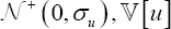 is replaced by
 . Notice that, due to the fact that λ relates the variance of the perturbance fromthe inefficiency term (u) with the variance of the white noise perturbance (6) not with the total production measured; its value is not directly associated with the production inefficiency but with the global system inefficiency; i.e., the value of λ is affected by the capacity of the production function to predict the optimal production. Hence, in order to determinate the pertinence of applying an SFA, previously we must check if the available data provided enough statistical power to perform the testing,
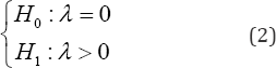
In practice, model (1) is transformed to obtain a new model in which, as usual, a zero-mean perturbance is involved,
Where,  . Both least square error (LSE) and ML methods perform adequately on this model. In fact, both procedures provide similar and good estimations for the parameters
  Hence, in practice, since the above parameters have been estimated, the obtained residual,(ε =){e1.....,,eN }(Nstands for the available sample size), can be considered as a random sample drawn from
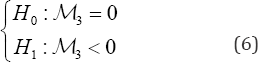
  Assuming that, under the null (λ=0),
  symmetrically distributed, a positivein probability λ-value should produce a decreased on the probability that s takes negative values. Note that this probability can be directly estimated from
  and 0 otherwise). Therefore',=applying the traditional sign test, we first propose to check the contrast in (2) from
 Despite the dependence among elements of
  because
  Where, Y is the vector of N observation from Y and
  is the orthogonal subspace projection matrix over the N observations of
  , under the null,
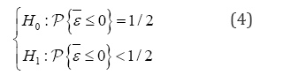
  could be approximated by a B(N,1/2) (binomial distribution with parameters N and 1/2 and then, for a fixed nominal level α,
Where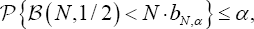 is an approxiated critical region for the contrast (4) at level α
When, as usual, it is assumed that o follows a symmetric distribution is also derived
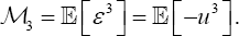 that Since, in the stochastic frontier model context λ > 0,(m3<0) the contrast in (2) two be the contrast
Besides, for residuals normally distributed, the Central Limit Theorem (CLT) and the Slutski�fs Lemma guarantee the following result
Theorem 1: Let {e1,...eN} be a random sample from
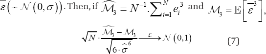
Where is a estimator for σ satisfying
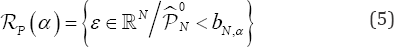
 in probability. Hence, the set
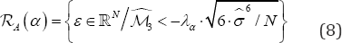
Where, is an (asymptotic) critical region for the contrast (6) at level α . It is worth to note that the asymptotic normality for the estimator
  can be proved under weaker conditions; however, parametric models must be assumed in order to approximate its variance.
Confidence intervals
Once it has been decided that, for the studied dataset, a stochastic frontier is the appealing appropriate model (this decision can be taken even when the null (2) is not rejected; in fact, in order to estimate the involved parameter, we only need that  the question of the "wrong" skewness deserves some discussion which was included in final section), the next step is to estimate the involved parameters and computing the respective confidence intervals. Usually, some parametric model is assumed at this point. In this section, we use the
  properties to make inferences on �f for the normal-half normal model and, from Monte Carlo simulations, it is studied the behavior of the obtained expressions.
Under the normal-half normal model, it is well-known that, for each , the the distribution function of the composite disturbance Ò-u is,
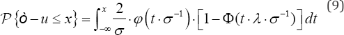
 and Ö stand for the density and the distribution functions of a standard normal law, respectively. Then, we have that
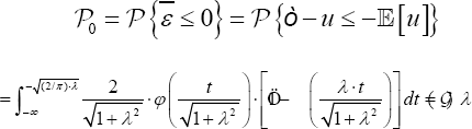
i.e., p0. only depends on the λ. values. In addition, follows again approximately a B (N,g(λ)) distribution, if IN,α/2 and SN,α/2 are the lower and the upper bound of a confidence interval (at level1-α) for
  then
then  and.
and. are the upper and the lower bound of a confidence ,interval (at level ) for λ. Of course, bootstrap methods can also be used in order to improve the variance estimation. Unfortunately, the function
  cannot be directly computed and, with this goal, numerical methods must be used. Figure 1 depicts the numeric computation for the function G.it is not defined for
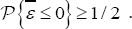

As it is well-known, the value of λ can also be derived from the M3 parameter. Particularly, it holds the following relationships:
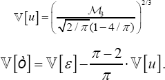
Therefore, for  can be directly estimated by using a plug-in method.
Monte carlo simulations
The practical behavior of the methodology exposed above is studied via Monte Carlo simulations. Three different scenarios have been considered. The first one is a simple normal-half normal situation; a sample with size ,N,X is drawn from a standard normal distribution and then, it is computed  where Ò follows a standard normal distribution and
  null 0,5,1,2,4 The second scenario, contaminated normal-half normal, is similar to the previous one but, approximately, the 2.5%of the data are contaminated by a perturbation following the mixture 1/2. N(-3,0.1) +1/2. N(3,0.1). Note that, in this scenario, the distribution of the white noise,Ò is not exactly a N(0,1) but, approximately, the mixture 0.0125 N (-3,0.1) + 0.975 o N (0,1) + 0.0125 o N (3,0.1). Finally, in the third scenario, we consider a model with one dependent variable and three regressors the covariance matrix and the linear regression model structure as well as the total variance of the residuals are based on the WHO data adding a normal-half normal perturbation (complete information of this dataset is provided as Appendix).
Hypothesis testing
In this subsection, we investigate the capacity of the previous tests for detecting the presence of skewness under the three scenarios described above. Results based on 5,000 Monte Carlo iterations for the tests based on regions (5) (P0) and (8) (Sk)by using the standard Wald-based method, W(the R package frontier was used with this goal) and by a simple analysis of the residuals normality using the traditional Shapiro-Wilks test (S - W) are provided in the following tables and figures. Table 1 shows the rejection proportions for the normal-half normal model when X = 0 (null) at nominal levels α = 0.05 and α = 0.10. Nominal levels were respected by P0, Sk and (S-W) methods but, the standard W test obtained catastrophic results; at level α = 0.05 between 12.8% and 21.5% of samples were rejected.


Figure 2 shows the observed rejection proportions for the four considered tests for λ2 = 1/2,1,2 and 4 . Logically, the Wald test is always the best one; it obtained a good power even for λ = 0. It is followed by Sk and S - W . The new introduced test, P0, obtained the worst results. Note that even for λ = 1 and N=1,000 the Observed power does not achieve 80%. Table 2 shows the observed rejection proportions for 5,000 Monte Carlo iterations under the scenario 2 (contaminated normal-half normal). All considered test overestimated the nominal level. Logically, Shapiro-Wilks test increases the rejection proportion with the sample size; note that, in this case, the null hypothesis is not true because the residuals are normal distributed. However, test based on P0 shows itself more robust than the others; at level α = 0.05, it rejected a maximum of 8.3% (N=100) and around the 6% when sample size increases. The rejection proportion for the tests based on Sk and W increased with the sample size to achieve the 20.3% and 60.5% for N=5,000 and α= 0.05, respectively.


Figure 3 is similar to Figure 2 for the contaminated normalhalf normal scenario. Because, at this scenario, it does not hold the residuals normality even for ë = 0, the Shapiro-Wilks test has not been included in this plot. The Wald test was, again, the most powerful one; remember that the rejection proportion under the null was also really high. Tests based on Sk and P0 had similar behaviour although S was always better than P0. Finally, Table 3 shows the observed rejection proportions, under the null, for the third considered scenario. Tests based on P0, and Sk, and S — Wrespected the two considered nominal levels. However, the Wald test increased the rejection proportion with the sample size, even it overcame the 50% for N=5,000and a=0.05. Figure 4 shows the observed power for the four studied tests in the third described scenario. The results were not essentially different to the ones observed in Figure 2. However, it is worth to remark that, in this scenario which is more complex than the previous ones, for λ2 = 1/2,1,2, the Wald test worked worse than Sk and, for the largest X, even worse than the Shapiro-Wilks and P0 tests. In addition, P0 shows itself more competitive since it is not affected for the new scenario.
Confidence intervals
In order to study the quality of the estimation provided by the skewness based methods and the usual maximum-likelihood based one, we explored the coverage percentage of symmetric 95% confidence intervals built by using the usual naive bootstrap method (200 replications) for the procedures based on the probability (p) and (Sk) the moments . In addition, the R package frontier is used to compute the confidence interval for the maximum-likelihood method. Table 4 shows the observed results in 5,000 Monte Carlo iterations from the scenario 1. Obviously, estimations have only been computed when it was possible (final sample used is provided as % valid). With the coverage percentage, the length of the 95% confidence interval is reported by mean ± sd (standard deviation). Results show that only the P estimator achieved the expected coverage percentage in all situations. Sk an W estimators obtained really poor results for small sample and mild X — values. The W estimator directly cannot be used for λ2 lower than 1 andif X2 = 1 sample size must be really large. Table 5 is similar to Table 4 when samples are drawn from scenario 2. The three considered tests obtained bad results in this setting. Sk and Westimators achieved really poor coverage. These results were only similar to the expected ones for λ=2. In addition, the coverage percentage decreased with the sample size for the three investigated estimators. In spite of the length of the respective confidence intervals were the largest, only P0obtained reasonable results for most of the considered situations. Table 6 shows the observed results for the scenario 3. These results were not different to the ones obtained in Table 4. Usual estimator based on the maximum-likelihood ratio only worked for


Real data analysis: the WHO data
In order to illustrate the practical behavior of theinvestigated estimators, the well-known data from the World Health Organization (WHO) is studied [17]. Particularly, we consider data referred to the year 1997 with a total of 227 world regions (N= and we try to model the Disability Adjusted Life Expectancy (DALE) from the regressors: per pro-capita health expenditure (HEXP) and educational attaintment (HC). Last variable is considered in quadratic form and therefore the regressor HC2 (square of the educational attaintment) is also included in the model. Since the logarithm transformation is usually applied, the standard square error method provides the equation, Where,
  hence based on the probability estimator, and assuming the normal-half normal model
  =0.874; the p-value associated with the null was 0.629. On the other hand,
  =0.003;the p-value associated with the null :H0:m3=0 was 0.929. The value of too close to zero and does not allow to estimateλ>0The maximum-likelihood based procedure provided a λ
estimator of 5.76 with a p-value=0.001. The parameters werealso slightly different and the obtained equation was,
=0.003;the p-value associated with the null :H0:m3=0 was 0.929. The value of too close to zero and does not allow to estimateλ>0The maximum-likelihood based procedure provided a λ
estimator of 5.76 with a p-value=0.001. The parameters werealso slightly different and the obtained equation was,
Figure 5 depicts the densities for the model based on the maximum-likelihood with residuals normal-half normal distributed  forλ=0 normal residuals and kernel density estimation for the observed residuals. Although it seems that the residuals are not drawn from a normal law Shapiro-Wilks test rejects this hypothesis with a p-value=0.001, the kernel density estimation (KDE) is far from the normal model but also far from the normal estimator of the maximum like lilehood method

Discussion
Stochastic frontier models are conventionally used in order to study production and cost functions. The specialized literature focuses are, mainly, the estimation of the parameters of these functions by regression techniques. Parametric normalhalf normal residuals joint with the maximum-likelihood method is, probably, the most frequently employed procedure. In the voluminous literature on this topic, statistical testing of the properties of the disturbance term has attracted little attention. In this work, the authors deal with the stochastic frontier model identification from a statistical approach. Via Monte Carlo simulations, we study the performance of the Wald test computed from the R package frontier. The results were catastrophic; Wald test respects neither the nominal levels nor the coverage percentages in most of the considered situations. Moreover, in the outliers' presence, the obtained results were extremely poor. These results support previous works which achieved similar conclusions [11,14].
Similarly, to Kuosmanen & Fosgerau [15], we proposed to study the residuals expected skewness in order to make inference about the data capacity to establish a stochastic frontier model. In spite that Simar and Wilson [16] and Feng et al. [18] worked on the so-called "wrong" skewness and it seems clear that, even when the stochastic frontier model is correctly specified, data can present "wrong" skewness. We assume that, in these cases, data have not provided enough evidence to estimate the potential SFA.The new proposed estimator, based on the expression  is really easy to compute, fully non-parametric and very robust, which implies being a bit conservative when there is not outlier in the sample. The analysis of the considered real dataset was
really enlightening; while _A4, estimator provided a really close
to zero estimation,
is really easy to compute, fully non-parametric and very robust, which implies being a bit conservative when there is not outlier in the sample. The analysis of the considered real dataset was
really enlightening; while _A4, estimator provided a really close
to zero estimation,  obtained a λ estimation close to 1 (it was poor taking into account the available sample size and the power observed in the Monte Carlo study). The Wald method provides
a λ value larger than 5. The observation of the residuals distribution suggests a lack of normality in their distribution, but the adjustment to the normal-half normal model proposed by the maximum-likelihood method was even worse. It seems that the maximum-likelihood method assigns all deviation from normality to the so-called inefficiency; however, as it is well- known, a regression model can have different problems which produce a lack of normality in the residuals distribution.
obtained a λ estimation close to 1 (it was poor taking into account the available sample size and the power observed in the Monte Carlo study). The Wald method provides
a λ value larger than 5. The observation of the residuals distribution suggests a lack of normality in their distribution, but the adjustment to the normal-half normal model proposed by the maximum-likelihood method was even worse. It seems that the maximum-likelihood method assigns all deviation from normality to the so-called inefficiency; however, as it is well- known, a regression model can have different problems which produce a lack of normality in the residuals distribution.
In short, stochastic frontier models frequently try to detect a slight deviation in the normality of the residuals; this deviation is assigned to the inefficiency term. However, detecting these deviations is really difficult without huge samples. In addition, the origin of these deviations cannot be the inefficiency term; in particular, there exists different causes which provoke this effect. A deep study of the residuals distribution, particularly of their symmetry can drive to obtain a good knowledge about the real nature of the model. Of course, the application of (relatively) modern techniques to analyzed the symmetry of the perturbance distributions or methods based on quantiles among many others can be useful [19,20].
Acknowledgement
First author has been supported by grant of Erasmus Mundus MEDASTAR (Mediterranean Area for Science Technology and Research) program, 2011-4051/002-001-EMA2. The authors acknowledge support by the Grants MTM2015-63971-P and MTM2014-55966-P from the Spanish Ministerio of Economía y Competitividad, FC-15-GRUPIN14-101 from the Principado de Asturias and Severo Ochoa BP16118 (this one for Pérez- Fernández).
References
- Aigner D, Lovell CAK, Schmidt P (1977) Formulation and estimation of stochastic frontiers production function models. Journal of Econometrics 6: 21-37.
- Meeusen W, Van den BJ (1977) Efficiency estimation from Cobb- Douglas production functions with composed error. International Economic Review 18: 435-444.
- Fan Y, Li Q, Weersink A (1996) Semiparametric estimation of stochastic production frontier models. Journal of Business and Economic Statistics 14: 460-468.
- Martins-FC, Yaoc F (2015) Semiparametric Stochastic Frontier Estimation Via Profile Likelihood. Econometric Reviews 34(4): 413451.
- Kumbhakar SC, Park BU, Simar L, Tsionas LG (2007) Nonparametric stochastic frontiers: A local likelihood approach. Journal of Econometrics 137(1): 1-27.
- Greene WH (1993) The econometric approach to efficiency analysis, In: Fried HO, Lovell CAK, Schmidt SS (Eds), The Measurement of Productive Efficiency, Oxford University Press, New York, USA, pp. 68119.
- Stevenson RE (1980) Likelihood function for generalized stochastic frontier estimation. Journal of Econometrics, 13: 57-66.
- Greene WH (1990) A gamma-distributed stochastic frontier model. Journal of Econometrics 46: 141-163.
- Schmidt P, Lovell AK (1979) Estimating technical and allocative inefficiency relative to stochastic production and cost frontiers. Journal of Econometrics 13: 83-100.
- Simar L, Van Keilegom I, Zelenyuk V (2014) Nonparametric least squares methods for stochastic frontier models, Working paper series; Centre for Efficiency and Productivity Analysis.
- Coelli TJ (1995) Estimators and hypothesis tests for a stochastic frontier function: A Monte Carlo analysis. Journal of Productivity Analysis 6: 247-268.
- Olson JA, Schmidt P, Waldman DM (1980) A Monte Carlo study of estimators of stochastic frontier production functions. Journal of Econometrics 13: 67-82.
- Behr A, Tente S (2008) Stochastic frontier analysis by means of maximum likelihood and the method of moments, Discussion Paper Series 2: Banking and Financial Studies.
- Simar L, Wilson PW (2009) Inferences from cross-sectional stochastic frontier models. Econometric Reviews 29(1): 62-98.
- Kuosmanen T, Fosgerau M (2009) Neoclassical versus frontier production models? Testing for the skewness of Regression Residuals. Scandinavian Journal of Economics 111(2): 351-367.
- Wilson PW (2008) FEAR: A software package for frontier efficiency analysis with R, Socio-Economic Planning Sciences 42(4): 247-254.
- Evans D, Tandon A, Murray C, Lauer J (2000) The comparative efficiency of national health systems in producing health: an analysis of 191 countries. World Health Organization, GPE Discussion pp. 29.
- Feng Q, Horrace WC, Wu GL (2013) Wrong skewness and finite sample correction in parametric stochastic frontier models, Center for Policy Research Maxwell School of Citizenship and Public Affairs Syracuse University, USA.
- Ahmad IA, Li Q (1997) Testing symmetry of an unknown density function by kernel method, Nonparametric Statistics 7(3): 279-293.
- Staudte RG (2014) Inference for quantile measures of skewness. Test 23(4): 751-768.


