


The Analytical Covariance Matrix for Regime - Switch in Models
Andrea B*and Benedikt R
Department of Economics, University of Munster, Germany
Submission: September 12, 2017; Published: November 16, 2017
*Corresponding author: Andrea Beccarini, Department of Economics, University of Munster, Germany, Email Andrea.Beccarini@wiwi.uni-muenster.de
How to cite this article: Andrea B, Benedikt R. The Analytical Covariance Matrix for Regime - Switch in Models. Biostat Biometrics Open Acc J. 2017; 4(1):555626. DOI: 10.19080/BBOAJ.2017.04.555626
Abstract
This letter provides an analytical solution for the covariance matrix related to the (mean) parameters of the standard Markov-switching model. The importance of avoiding numerical procedures to estimate this matrix is also highlighted. Simulations are also performed in order to verify, in small samples, the actual advantage of the analytical formula
Keywords: Regime-switching; Covariance matrix; Simulations
Introduction
The seminal paper of Hamilton [1] provides a very attractive way to estimate regime-switching parameters of a model where the latent variable governing the regime switching enters the model without its lags. In this case, closed form solutions for these estimates are available. Surprisingly, Hamilton and the subsequent applied and theoretical literature do not consider a closed form solution for the related covariance matrix. Thus, the covariance matrix is generally found by numerical procedures whose aim is generally to estimate both the point Markov- switching (M-S) estimates and their covariance matrix in the maximum likelihood (ML) framework.
However, in this context, the use of numerical procedures for finding point estimates and the related covariance matrix are not efficient. In fact, point estimates are found by closed form solutions. Consequently, having available an analytical calculation for the covariance matrix casts doubts on the rationale of the application of numerical procedures. They turn out not only to be inefficient with respect to their analytical counterparts but also ineffective as they are based on approximations.
Now, the estimator based on numerical procedures suffers from a certain degree of approximations, involving sometimes unstable and cumberosme calculations. In fact, once considering the Newton-Rapson algorithm as a reference numerical procedure, it can be shown that, this algorithm works well only when the log-likelihood function is quadratic [1]. Furthermore, at points distant from the optimum, the second derivative matrix may not be negative definite [2]. However, alternative methods to the Newton-Rapson’s partially solve these kinds of problems For example, the Davidon-Fletcher-Powell algorithm (Quasi-Newton method) overcomes the latter problem by eliminating the second derivatives altogether from the calculations, leaving the researcher with the need to separately estimate the covariance matrix. In order to overcome these problems, we propose an analytical estimate of the covariance matrix in question. We also show that, for small samples, the precision of our estimator is quite larger [3,4]. The reminder of this letter is organized as follow; the next section shows how to derive the analytical solution for the covariance in question; section three shows some simulations. Then conclusions follow.
The analytical solution
The model of Hamilton [1] can be rewritten in matrix notation:
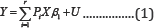
Such that,
A1. Y is N x1 vector of observations drawn from the dependent variable yn (n=1,....,N ).
A2. X is a matrix including in the first column a vector of ones and K vectors of observations drawn from K exogenous explanatory variables xn,j (J =1,---,K and n = 1,.,N)
A3. plim Where, Q is a (K + l)x(K +1) matrix of finite random elements.
A5. The latent polytomous variablePn = 1,...r, (withn=i,...,N) defines the regime occurring for the nth-observation. The observations of the variables pn are conveniently organized in r diagonal (NxN) matrices, pi , such that the n-th element of the diagonal is 1 if the n-th observation belongs to regime i and 0 otherwise
A9. U is a Nx1 vector of disturbances drawn from un∼NID(0,σ2)n=1,......N, independent of X and of P (i = 1, 2,..., r) It also holds that: plim 
Under these assumptions, we may now define the M-S estimators as the estimators based on the EM (Expectation- Maximization) algorithm, as:
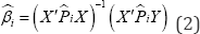
Where,  is a NxN diagonal matrix embedding in the main diagonal the estimated smoothed probabilities of regime and for each observation. In fact, considering the first-order condition (FOC) related to the parameter βi one has:
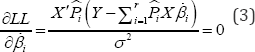
Where, LL is the expected log-likelihood maximized at the M-step. Under the condition that regimes are separated  see Ruud [5], one has (p)
 thus the solution of the above FOC is Eq.(2).
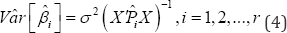
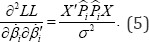
Now, we show how to derive the analytical covariance matrix formula. In fact, by twice differentiating the expected log- likelihood LL, with respect to the parameter vector one obtains the expression:
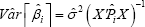
Proposition
Proof: Considering the FOC of the Log-likelihood and deriving that again with respect to one obtains
Since, the elements of the off-diagonal of the Information matrix are zero, in expectation, it turns out that:
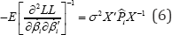
Having assumed that regimes are separated implying that 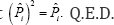
Simulations: In this section, we provide a Monte Carlo analysis of the proposition in Eq. (4) to investigate the sensitivity of the analytical and the numerical covariance matrices in small and large samples. We consider the simple univariate model of Eq. (1) with r = 2 regimes:

The explanatory variable X is assumed to follow a simple white noise process. According to A9, U is a Nx1 vector of disturbances drawn from un∼NID(0,σ2) for n = 1,..., N βi is a2 x1 coefficient vector containing an intercept αi and a slope parameter θi for each regime i with i = 1,2 Furthermore the probability that regime 1 will be followed by regime 1 is given by p( pn= 1 |Pn-1 = 1) = 0.9 and the probability that regime 2 will be followed by regime 2 is given by p( Pn =2| Pn-1 =2) = 0.7 Table 1 shows the parameter specification of the model in Eq. (7). This specification takes into account the condition that the regimes are separated, that is

We run our Monte Carlo analysis with 5000 replications and use a small sample of N = 50 and a large sample of For n = 500 each simulation we compute the point M-S estimates and their covariance matrix in the ML framework as well as the point estimates  based on the analytical formula in Eq. (4). To compare the results, we compute the mean values over all replications of the estimated covariance matrix, based on the numerical procedure and based on our analytical formula. For the sake of simplicity we concentrate on the estimated variances of the four parameters. The results are given in Table 2. In both samples the mean values of the analytical variance are smaller than numerical variances. In small samples (N = 50), the approximation implied by the numerical procedure is large as the differences between the analytical and the numerical variances of the parameter estimates are sizeable. In large samples (N = 500), the mean values of both variance estimates decrease but the differences between the variance estimates are negligibly small. Based on these results, we conclude that, for small samples, the precision of our estimator is quite larger.
Conclusion
In this letter we have shown how to find an analytical formula for the covariance matrix of point estimates of a standard Markov-switching model. This formula is derived directly from the closed form solution obtained in Hamilton [1], for the point estimates. Having in hand a closed form solution avoids the application of numerical procedures in the M-step of the EM algorithm; in so doing, it eliminates the potential problems related to the numerical procedure and fastens the global convergence of the EM algorithm. Simulations show that, in small samples, the approximation implied by the numerical procedure is large as the difference between the analytical and the numerical covariance matrices is sizeable.
References
- Hamilton JD (1990) Analysis of time series subject to changes in regime. Journal of Econometrics 9: 27-39.
- Greene WH (2012) Econometric Analysis (7th edn), Pearson.
- Hamilton JD (1994) Time Series Analyisis, Pricenton University Press, USA.
- Hamilton JD (1996) Specification Testing in Markov-Switching Time-Series Models, Journal of Econometrics 70(1): 127-157.
- Ruud P (1991) Extensions of estimation methods using the EM algorithm. Journal of Econometrics 49: 305-341.