


Multiple Imputations for Determining an Optimum Biological Dose of a Metronomic Chemotherapy
Atanu B*, Gajendra V, Jesna J and Ramesh K
*Centre for Cancer Epidemiology,The Advanced Centre for Treatment, Research and Education in Cancer (ACTREC),Tata Memorial Centre, Mumbai, India
2Department of Applied Mathematics, Indian Institute of Technology -Dhanbad- 826004, India.
3King Abdullah International Medical Research Center (KAIMRC),King Saud Bin Abdulaziz University for Health Sciences,Ministry of National Guard-Health Affairs,Riyadh,Kingdom of Saudi Arabia.
Submission: August 23, 2017; Published: October 24, 2017
*Corresponding author: Atanu Bhattacharjee, Department of Statistics, Gauhati University, Guwahati, India; Email: atanustat@gmail.com
How to cite this article: Atanu B, Gajendra V, Jesna J, Ramesh V. Modeling the Infant�s Age at Hospital Admission in Neonatal with Jaundice at the Ghaem 02 Mashhad Hospital Using Count Models with Excess Zeros. Biostat Biometrics Open Acc J. 2017; 3(5): 555621. DOI: 10.19080/BBOAJ.2017.03.555621
Abstract
The doses of chemotherapy selected in clinical practice are routinely derived by the Maximum Tolerated Dose (MTD) approaches. It is believed that an increase in dose will lead to an increase in tumor response. The effect on angiogenesis is achieved by targeting Circulating Endothelial Cell(CEC). The effect on CEC is restricted to an antiangiogenic window in tumor cell line studies The challenge is to establish the optimal biological dose (OBD) of MC which would have maximized inhibiting effect on CEC. The inhibiting effect of CEC is required to measure with repeated manners and can be considered as Surrogate Marker of Angiogenesis. There is no consensus on the most appropriate approach to surrogate marker response with effective metronomic chemotherapy. Therefore a simulation study was performed to assess the OBD on the performance of a MC. Datasets were generated to resemble the skewed distributions seen in a motivating head and neck cancer (HNC) example. The CEC count is considered as time dependent surrogate marker. The joint distribution with the time-to-event and longitudinal outcomes are considered. The missing data mechanism is defined through consideration of conditional distribution of the time-to-dropout condition to the complete vector of longitudinal outcomes. The parameters of interest are estimated through Bayesian approach on joint modeling.
Keywords: MTD; CEC; OBD; Missing; Joint Modeling; Time=to-Event
Introduction
The doses of chemotherapy selected in clinical practice are routinely derived by the Maximum Tolerated Dose (MTD) approaches. It is believed that an increase in dose will lead to an increase in tumor response. The dose selected for phase 2 and further studies is one dose level below the MTD level in Phase I studies [1-3]. However, this conventional dosing of chemotherapy has routinely compromised the QOL of patients and may lead to selection of chemo-resistant clones [4-6]. The Metronomic Chemotherapy (MC) has been suggested as an alternative strategy to overcome such effects. The strategy in MC is to administer subtoxic doses (i.e.nearly of MTD) of same chemotherapy drugs for long periods to target angiogenesis [7-10]. The effect on angiogenesis is achieved by targeting Circulating Endothelial Cell(CEC). The effect on CEC is restricted to an antiangiogenic window in tumor cell line studies [1,11,12].
In tumor cell line studies a drug would start exerting an antiangiogenic effect at a low dose level and it would continue to exert it till an upper dose level. Drug levels below the lower dose level and above the upper dose level won't exert an antiangiogenic effect. The challenge is to establish the optimal biological dose (OBD) of MC which would have maximized inhibiting effect on CEC. The inhibiting effect of CEC is required to measure with repeated manners and can be considered as Surrogate Marker of Angiogenesis [13]. The failure to achieve inhibiting effect of CEC proceeds to the recurrence of tumor and further death to a patient. The bridged problems are determination of OBD of MC through consideration of repeatedly measured CEC maker's values on time-to-event data. However, in this paper we will concentrate on reasonably two best performing OBD and their effectiveness to maintain continuously measured CEC maker's values on angiogenesis and further time-to-event rate among the treated patients with specific MC dose.
Methods
The simulation techniques adopted within this study are given below. All simulations were carried through the freely available R statistical software, thus allowing all researchers access to any suitable methods identified.
Generating the datasets
There is no consensus on the most appropriate approach to surrogate marker response with effective metronomic chemotherapy. Therefore a simulation study was performed to assess the OBD on the performance of a MC. Datasets were generated to resemble the skewed distributions seen in a motivating head and neck cancer (HNC) example. The CEC count is considered as time dependent surrogate marker. The baseline CEC count in the blood of HNC patients incorporated from normal distribution (with mean 114 CEC per ml; SD 15) for a total of 220 patients. The dose 1 and dose 2 are considered as OBD in this work with simplicity [14]. However, it is possible to consider several doses and obtain the best performing optimum dose based on the controlled level of surrogate marker i.e. CEC. The ID's of 200 patients were randomly assigned to the dose 1 and dose 2 with metronomic chemotherapy from the binomial distribution. The baseline measurement of four covariates named with ECOG (coded 0 and 1), HB Level(<12 and 12), Tumor size (mean 4:0 cm; SD 2) and Histological grades (well, moderate and poor)were generated randomly for a total of 220 patients and merged with the excel sheet. The ECOG, HB level and Histological grade were generated from binomial and multinomial distribution respectively.
The baseline tumor sizes were obtained through normal distribution. Further, the five follow-up visits observations for CEC and tumor size were assumed to be distributed with normal distribution. The mean value for CEC at time points t1; t2; t3; t4; t5 were assigned with mean 124,128,135,126,120 respectively. The SD was considered for each time points of CEC values to be generated as random measurements. The tumor size assigned with mean 4:0; 3:4; 3:2; 3:0; 3:2 with SD (2) for the time points t1; t2; t3; t4; and t5 respectively. The continuous covariates were postulated with a linear effect on the log relative hazard. An exponential distribution with a hazard rate of 0.0003 was considered to generate the uncensored survival duration. It is approximated with the hazard rate in the HNC [15]. The censored duration was also generated from the exponential distribution with a hazard rate of 0.0003 with approximately 45% censored observations. The required survival duration was defined for each cases as the minimum of the uncensored and censored survival duration and the event status defined accordingly. The recurrence is considered as event of interest. The survival duration is represented as progression free survival (PFS).
Model
The ith subject's longitudinal measurement at time point t is denoted as Yi(t). Further, the time to occurrence of event is defined as T and Ci respectively. The term Ti and Ci are defined as time to outcome-dependent and outcome- independent dropout respectively. The measured data is defined Yij = {Y (tij) , j = 1,..... ,ni}, as for the specific time point tij It is assumed that, Ui = min(Ti,Ci), the observed event time, and the corresponding event indicator, and the measured observation is defined as Yij = {y (tij), j = 1,.....,ni}, the longitudinal responses at specific occasions tij at which measurements were taken. The subject-specific longitudinal trajectories is defined as
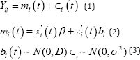
In equation (2) the term xi (t) is used as fixed effects for the β and zi(t) as the random effects bit . The error terms are time-dependent and assumed that the errors are mutually independent with random effects. The random error is assumed with normally distributed with mean zero and variance σ2 . Thereafter, we will give emphasize on mi (t) as a component of Yi (t). The risk of event is defined as
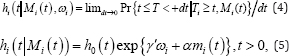
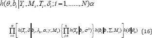
The unobserved longitudinal process up to time point is defined as Mi (t) = {mi (s),0 ≤ s ≤ t}. The baseline risk function and covariates are defined as h0 (.) and with regression coefficients γ . The parameter α is used to facilitate the effect of the underlying longitudinal outcome on the risk for an event. The relative change in the risk for an event at time t is covered through exp(α) as one unit increase in mi (t) at the same time point. It shows that the relative risk for an event at time t depends only on the current value of the time-dependent marker mi (t). It stands that the survival function depends on the whole longitudinal response history Mi (t) , Mi(t),through the relation between the survival function and the cumulative hazard function, i.e.,

The estimation of (t) is dependent on the estimation of Mi (t) . Therefore, it is important to specify the time dependent structure in xi (t) and zi (t) can be considered with highdimensional vector of functions with time t. The splines as a vector of choice is preferred due to their numerical suitability and local nature [16]. The spline based approach is already adopted and found suitable like B-splines with multidimensional random effects [17,18] and cubic splines [19]. The joint model is defined as
Yi(t)=mi(t)+∈i(t)(7)
It is assumed with u (t)i is independent with bi and it follows mean-zero with stochastic process. The error term ∈i (t), and mi(t) has the mixed-effects model structure as defined in equation (1) and (2). The latent stationary Gaussian process through shared processes [20] and Ornstein-Uhlenbeck Process [21] on joint modeling have adopted and those approaches found appropriate with different dynamic biological scenario that generated with data. The subject specific trajectory is dedicated through time independent random effects bi alone. It involves that the shape of the longitudinal pro le of each subject is natural feature of this subject that is constant in time. It is possible to generate indistinguishable fits to the data, if the serial correlation term ui(t) has not been addressed properly by random-effects structure under the consideration of linear mixed model. However, it is difficult to address random effect and serial correlation simultaneously through a single model. It is easier to consider with random-effects by design matrix zi. It is natural practice to avoid the consideration of specific distribution for the function h0 (.) of to withdraw the impact of misspecifying the distribution of survival times. Incase of joint modeling it leads to underestimate of the parameter of interest[22] . It is required to define h0 (.). It can be linked with risk function corresponding to an know parametric distribution or flexible parametric distribution at baseline risk function [23-25].
The objectives of this study raised the challenges. For instance, the subject with controlled CEC value may have controlled tumor growth, having lesser risk of recurrence and relatively lesser risk of death due to cancer. It can be defined as "nonignorable" missing data [26,27]. The generic attempt is to apply longitudinal data model through consideration of CEC value changes, but it may generate biased estimates. The Cox PH model can be considered to explore the relation between CEC value (i.e. as time-dependent covariate) and time to recurrence or death, when the true CEC trajectory  value is known to us. There are two more challenges. First, the CEC value is prone to be affected with considerable amount of measurement error due to both biological variability and presences of laboratory. The widely used method is to substitutes the observed time- dependent covariate for the true covariate values in the PH model. However, this method can leads to biased estimates of the relative risk parameters and it can leads towards biased estimates of the relative risk parameters on measurement error [28,29]. Secondly, the CEC value observed intermittently, it is not feasible(due to costly procedure) to repeatedly measured at the exact time when failure event occurs for the individual in corresponding risk group. The normal procedure is to consideration of "Last Observation Carry Forward (LOCF)" as a representative of future CEC value from past measurement.Although it is not robust procedure because time to event and corresponding true CEC value will not be there to be correlated.
The LOCF method fails to consider the measurement error, it also overlooks the possible trend of the CEC, resulting very inferior inputs about missing markers values. It leads to poor estimates of the relative risk of parameters. The measurement error can be handled with smoothing technique. The regression calibration is suitable to capture the available trend of the covariates over time and thereafter impute the missing values of covariates for individuals at risk. The imputed values can be adopted in the disease risk model if they are fitting Yi* (t) at the time of each event. This procedure can be adopted through Cox PH model and mixed effect modeling. However, there are certain chances to get the biased results and the estimates of the risk parameters associated with the longitudinal data may not be true, particularly for the relatively sparse longitudinal data. We tried to attempt with joint modeling framework through consideration of longitudinal and time-to-event data analysis.The idea is to maximizing the likelihood [Ti, Yi|Mi ] in terms of covariate process and time-to-event data. The informative drop-out assumed to be adjusted with survival modeling, and thereafter unbiased information about the longitudinal covariates were included into the survival model. It helped us to make joint between the failure time with the longitudinal surogate marker. The joint modeling is attempted to build the robust estimates of the parameter through modeling [27,28].
Joint model
A separate term ni as unobserved latent variables is induced to define the relation between surogate marker
process and failure times on conditionally independent given with the baseline covariates Mi . The likelihood is formed with

It is required to specify the survival submodel [Ti , Yi|Mi ] ,longitudinal submodel [Yi|ni,Mi] and latent variable model ni separately to make relation between the two submodels.
Survival submodel
The survival submodel is defined as

The term λ0(t) used to define the baseline risk function, and q (.,..) is a vector function of time and the latent variables ni , γT are a vector of regression coefficients associated with baseline covariates Mi . The term q(t,ni) is used to define the joint model with Yi* (t) . It is assumed that the risk of event at time t depends only on the current value of the longitudinal process. There are different option to specify the distribution of the baseline hazard function λ0(t) under the parametric setup like (the Weibull, the log-normal, the Gompertz, and the Gamma distributions).
Longitudinal submodel
The continuous value of marker's (Yi*(t)) is defined through random effects as :
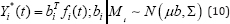
The term fi (t) is used to define as the function of time t for q elements. This equation further modified with through consideration of simple linear random effects model for f i(t) as
Yi*(t)=b0i+b1i (11)
The terms b1i and b0i are defined for slope and subject- specific random intercept respectively. It is feasible to consider random effects term bi as latent variable ni [19,17,30,18].
Joint Likelihood formulation and assumptions
The complete log-likelihood conditioned on baseline covariates Mi is defined as
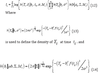
is adopted as density of the random effects bi and the part h(Tiδi|bi,λi,α,γ,Mi)is used as the density for the survival data. It is denoted as

The random effect part are latent and not observed, the log- likelihood for the observed data is defined as

It is assumed that the observed marker measurement Yi*(t) is dependent on the earlier time measurements
With {Yi1,...... Yik} (where tik<t). The latent random effects bi is considered free from the future time point measurement of Y-i(t).
It is also assumed that the observed marker history {Yi1,....Yik} (where tik < t ) and covariates Mi are independent with latent marker process Yi * (t) for time point t.
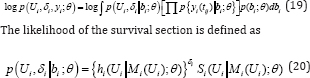
Bayesian methods
The parameters of interest are estimated through Bayesian approach on joint modeling. The prior distribution θ of is defined as h(θ|θ0 ) through the support of hyperparameters θ0 . The joint posterior distribution and latent random effects model is defined as
The unknown parameters and latent random effects were obtained through Markov chain Monte Carlo algorithm, using the Gibbs sampler [31-34].
The Gibbs sampling procedure provides the iterative sampling from the full conditional distribution of each
parameter given the current assignment of all other parameters and data. The convergence was assessed through the means, medians and variance of the Gibbs samples, and graphs of the empirical distributions. This procedure provide us to borrow strength from experts and incorporate this information in the current analysis and it also permit full and exact posterior inference for any parameter or predictive quantity of interest.
Estimation
The joint distribution with the time-to-event and longitudinal out comes is defined with p {ui ,δi, Yi}. It is assumed that the vector of time independent random effects bi is shared with longitudinal and survival procedure. The random effects part is used to make association between the time-to-event and longitudinal outcomes. The correlation between the repeated measurements is considered as conditional independence. It defined as
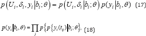
The term θ is the vector parameter, yi is the ni x1 assigned as longitudinal vector for the responses with ith subject, and p (.) provides an appropriate probability density function. It is assumed that the longitudinal and survival submodels both share the same random effects (the shared parameter modeling). The conditional independence assumptions of the joint log- likelihood contribution for the ith is defined as
The survival function hi(.) for p{yi (tij)|bi;θ} as the univariate normal density for the longitudinal responses, and p(bi;θ) is the multivariate normal density for the random effects. The log- likelihood function with respect to is a difficult. The challenge is integral with the random effects and define the survival function. However, the Monte Carlo has been attempted under the joint modeling approach [20,35,36] and there are further extension through Laplace approximation [17]. In this work, we attempted and considered the random effects to deal with 'missing data'.
Handling with missing data
The missing data mechanism is defined through consideration of conditional distribution of the time-to-dropout condition to the complete vector of longitudinal outcomes (yi0, yim ).
The observed part (consisted with all observed measurement) is defined as and the missing part is defined
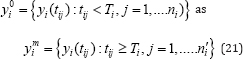
It includes the observed measurements taken until the end of the study. The dropout mechanism adopted under the joint model is
The NMAR technique is considered to define posterior distribution of the random effects p(bi|yi0,yim,θ) tohandle the time dependent dropout Yim. The single random effect (bi) component is adopted to address the survival and longitudinal sub-models jointly [37-39]. It is important to make relation between α and missing data procedure. The joint probability of the missing data and the longitudinal processes is defined as:
The defined parameter of the event time is defined with θ = (θt',θy',θb')' Further, the random effect part is
defined as θb and θy parameter for longitudinal outcomes. Initially, the parameters for the two submodel estimated separately. The log-likelihood for the longitudinal process is defined with It is also applicable for MAR and it is assumed that the dropout data is dependent on observed response. If it is assumed that α = 0 then it can served as MCAR mechanism.
The observed data under the consideration of log-likelihood of the complete data is defined as {yi0, yim} for the longitudinal outcome:
It is to be noted that the missing longitudinal processes yim is involved as the density of the longitudinal sub-model. Inca se the dropout is intermittently missing, then the likelihood of a joint model can be easily assigned without considering integration with respect to the missing outcomes. The subject's number of repeated measurement increases then the there is limited effect about miss-specification of the random effect on inference [40-42]. Suppose, in the longitudinal model mi(t) is linked with the risk of event at time point t with parameter α through the association. It is possible to consider different types of parameterization to link the longitudinal outcomes and risk of dropout.

The term f (.) is assigned as a function of the true level of the marker mi(.) , with the random effects bi and as extra covariates ωi2. The general formulation of α can potentially defined as a vector of the parameters.
Random-effect Component
The longitudinal sub-model through the consideration of the linear predictor of the risk model is defined as

Where is considered to make association between random effect and hazard rate function. It is assumed that the patients who have a lower size of tumor at baseline are more likely to increase in their longitudinal trajectories are less likely to experience the drop out. The random-intercepts and randomslopes incorporated longitudinal sub-model is defined as
yi (t) = β0 + β1t + bi0 + bi1t + ∈ (t) (27)
The relative risk sub-model with the time dependent slope is defined as
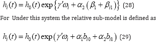
This model is flexible because if we consider , then the model provides the risk depends on the random-slopes component through linear mixed model.
Result
Markov chain Monte Carlo (MCMC) method which assumes multivariate normality has been used to impute
the missing values for all the variables in a data set with arbitrary missing data pattern. Haemoglobin, ECOG
grade and histological grade were used to impute the tumour size. Imputation of CEC values was done from
tumour size. The PROC MI statement is the required statement in the MI procedure for imputation. Available
options in the PROC MI statement are considered: METHOD=MCMC ,The CHAIN=MULTIPLE option, this
procedure uses multiple chains and completes the default 200 burn-in iterations before the single imputation.
The 200 burn-in iterations are used to make the iterations converge to the stationary distribution before the
imputation. The option INITIAL=EM was used to get the starting means and covariance from available cases to commence the MCMC process. The resulting imputed CEC values which are almost similar in both the groups in all visits are used for joint modelling, extended Cox-modelling and Cox regression analysis [43-45].

Table 1 summarizes baseline characteristics of patients receiving Metronomic Chemotherapy (MC). The baseline Haemoglobin level was less than 12 for 67(62:6%) patients in OBD dose level 1, whereas the baseline Haemoglobin level was less than 12 for 54(47:8%) patients in OBD dose level 2. The distribution of Histological grade is similar for both OBD dose levels. The number of patients with grade 0,1 and 2 are 21 (19.6) , 56 (52.3) and 30 (28.0) respectively in OBD dose level 1 where as the number of patients with grade 0 ,1 and 2 are 33 (29.2), 44 (38.9) and 36 (31.9) respectively in dose level 2. The Baseline ECOG grade is 1 for 72(67:3%) patients in OBD dose level 1 while it is 78(69:0%) in OBD dose level 2. The average (SD) value of Circulating Endothelial Cell (CEC) Biomarker is reported as 124.3 (15.44) in dose level 1 and 122.4 (15.46) in dose level 2. The average (STD) tumour size is reported as 3.6 (1.14) in dose level 1 and 3.4 (1.29) in dose level 2.
Table 2: describes the parameter estimates obtained through value has indeed a strong association with the risk for death for individual models and joint models. We observe that the CEC extended cox regression model.

In particular, a unit increase in the CEC value corresponds to a exp ( )=1.023 times increase in the risk for death (95% CI: 1.012,1.034). In the results for the event process for joint model, the parameter in (4.1) that measures the association between the true CEC value and the risk for death. The joint model also finds a strong association between the CEC value and the risk for death, with a unit increase in the marker corresponding to a fold increase in the risk for death (95% CI: 1.061,1.189). Comparing the point estimates and the corresponding 95% confidence intervals from the extended Cox model and the joint model, we clearly observe non-negligible differences. Table 3 summarizes the characteristics of patients receiving Metronomic Chemotherapy (MC) in each visit. At visit 5, Haemoglobin level was less than 12 for 32 (50.8) patients in OBD dose level 1, whereas the baseline Haemoglobin level was less than 12 for 33 (51.6)patients in OBD dose level 2. The number of patients with Histological grade 0 ,1 and 2 are 17 (27.0), 32 (50.8) and 14 (22.2) respectively in OBD dose level 1 where as the number of patients with grade 0 ,1 and 2 are 18 (28.1), 32 (50.0)and 14 (21.9) respectively in dose level 2.The ECOG grade is 1 for 47 (74.6)patients in OBD dose level 1 while it is 41 (64.1) in OBD dose level 2. The average (SD) value of Circulating Endothelial Cell (CEC) Biomarker is reported as 122.5 (15.77) in dose level 1 and 123.6 (20.01) in dose level 2. The average (STD) tumour size is reported as 2.7 (0.78) in dose level 1 and 2.6 (0.62) in dose level 2. The average (SD) value of Circulating Endothelial Cell (CEC) Biomarker was 124.3 (15.44), 136.8(15.34) , 151.9(16.11), 133.7(14.69) and 122.5(15.77) in visit 1 ,2,3,4 and 5 respectively in OBD dose level 1 while it is 122.4 (15.46),136.7 (16.38), 155.7(17.10), 136.8(18.64) and 123.6(20.01) in OBD dose level 2. The average (STD) tumour size was 3.6(1.14), 3.4(0.66), 151.9(16.11), 2.9(0.45) and 2.7(0.78) in visit 1 ,2,3,4 and 5 respectively in OBD dose level 1 while it is 3.4 (1.29), 3.3 (0.76), 155.7(17.10), 2.9(0.44) and 2.6(0.62) in OBD dose level 2 [46] (Table 3 (Visit 5)).


An interesting characteristic of the Metronomic Chemotherapy (MC) data is the unusual shapes of the subject specific longitudinal progresses. In particular, Figure 1 A & 1B to Figure 2 C & 2D, exhibit longitudinal profiles for all patients, Histological grade, Baseline Haemoglobin and Baseline ECOG. The solid lines depict the fitted subject-specific longitudinal profiles. Figure 3E, exhibit the Longitudinal response measurements for Biomarker for six randomly selected patients (a=101, b=129, c=211, d=144, e=155 f=179) from the Metronomic Chemotherapy (MC) patient study. The line depicts the fitted subject-specific longitudinal profiles based on the joint model. The patient profile demonstrates highly nonlinear longitudinal profiles for biomarker, which evidently cannot be effectively described by simple structures, such as linear or quadratic progresses in time. This specific problem motivated us to apply joint model that aimed to capture the characteristics of the dataset at hand and reveal related information [47].


To achieve this goal, we model flexibly the key components of the joint model while making standard parametric assumptions for the remaining parts. To further investigate the suitability of the chosen functional form for the CEC outcome, it is advisable to additionally check for systematic trends in the martingale residuals when we condition on other baseline covariates. Figure 4 (F) demonstrates Martingales residuals plot for subject -specific fitted values for overall treatment effect for Metronomic Chemotherapy (MC) patient study. Figure 4 (G) exhibits Martingale residuals versus the subject-specific fitted values of the CEC per dose level for the Metronomic Chemotherapy (MC) patient study. The black solid lines denote the fitted line. In this figure, Martingale residuals versus the subject-specific fitted values are displayed for dose level 1 on left side and dose level 2 on right side. An another type of residuals for survival models, associated to the martingale residuals, is the Cox-Snell residuals. For each subject, these are calculated as the value of the estimated cumulative survival function evaluated at the observed event time. This cumulative survival will have a unit exponential distribution. This identity implies that we can check the overall goodness-of-fit by checking whether the Cox-Snell residuals are exponentially distributed. In Figure 5 (H), The black solid line denotes the

Kaplan-Meier estimate of the survival function of the residuals (with the dashed lines corresponding the 95%
pointwise confidence intervals), and the red solid line, the survival function of the unit exponential distribution.


Figure 5 (I) demonstrates survival function for cox-snell residuals by dose level. The black solid line denotes the KaplanMeier estimate of the survival function of the residuals for each dose level, and the red solid line, the survival function of the unit exponential distribution. Figure 6 exhibits diagnostic plots, which is constructed to inspect the _t of joint models with reference distribution of the residuals for the longitudinal process is affected by the dropout. Figure 7 (K) compares the subject specific and Martingale residuals for fitted values.
Discussion and Conclusion
Low-dose chemotherapy drugs are more effective to suppress tumors by restraining tumor vessel growth and
preventing the repair of damaged vascular endothelial cells [48]. High dose chemotherapy drugs like Cisplatin
contributes to serious side effects [48]. The target of MC therapy is the vascular endothelial cells [47]. The growth of new vessels for a long run survival time treated with traditional maximum tolerated dose (MTD) through high dose chemotherapy has been confirmed [43]. The anti-angiogenic plays the important role as clinical potential. The metastasis and the growth of tumor cells depends on neovascularization [45]. The anti-tumor drugs could cause inhibition of tumor neovascularity [46].The low-dose chemotherapy drugs, as one- tenth of the MTD, administered continuously and frequently, could selectively suppress vessel growth in tumor tissues and prevent the repair of damaged vascular endothelial cells (VECs) [48]. This model is appropriate in dose-response modeling having the avoidable level of toxicity in any clinical trial. Based on our knowledge this is the first statistical methodological attempt that has been considered to deal with OBD with time- to-event and longitudinal data in MC trial. It is expected that this above mentioned methods will be useful for OBD detection in MC trials in future as well. The assumption about relation between missing data and unobserved longitudinal process is difficult [42,49]. Our proposed approach proceeds with random effect model. However, the random effect parts assumption and distribution is also difficult and there are previous attempt on that aspect as well. The random effect section is suitable to handle with flexible model through the class of densities [50], and semi-parametric estimation procedure [51]. However, there are some high amounts of standard error generation problem for miss-specification of parameter distribution. The results here suggest that metronomic chemotherapy can be efficacious in improving relapse free survival and survival, and have much less toxicity. This elaborated method can be considered to measure the effect CEC in long run improvement of overall survival (i.e., study initiation to death). This is an initial attempt to work with metronomic chemotherapy on this critical issue that still needs detailed exploration. This is a topic of current exploration. The results presented here to maintain the controlled level of CEC, can be extended to the desire level of PFS and OS through metronomic chemotherapy.
Declaration of interest
The authors declare that there is no conflict of interest that could be perceived as prejudicing the impartiality of the research reported.
References
- Skipper HE, Schabel FM Jr, Mellett LB, Montgomery JA, Wilkoff LJ, et al. (1970) Implications of biochemical, cytokinetic, pharmacologic, and toxicologic relationships in the design of optimal therapeutic schedules. Cancer chemotherapy reports 54(6): 431-450.
- DeVita, Vincent T, Chu E (2008) A history of cancer chemotherapy Cancer research 68(21): 8643-8653.
- Briasoulis E, Pappas P, Puozzo C, Tolis C, Fountzilas G, et al. (2009) Dose-ranging study of metronomic oral vinorelbine in patients with advanced refractory cancer. Clinical Cancer Research 15(20): 64546461.
- Schmid P, Walter S, Thorsten N, Gerdt H, Volker H (2005) Upfront tandem high-dose chemotherapy compared with standard chemotherapy with doxorubicin and paclitaxel in metastatic breast cancer: results of a randomized trial. Journal of clinical oncology 23(3): 432-440.
- Golfinopoulos V, Salanti G, Pavlidis N, Ioannidis JP (2007) Survival and disease-progression benefits with treatment regimens for advanced colorectal cancer: a meta-analysis. The lancet oncology 8(10): 898911.
- Saltz LB (2008) Progress in cancer care: the hope, the hype, and the gap between reality and perception., Journal of Clinical Oncology 26(31): 5020-5021.
- Hanahan D, Bergers G, Bergsland E (2000) Less is more, regularly: metronomic dosing of cytotoxic drugs can target tumor angiogenesis in mice. Journal of Clinical Investigation 105(8): 1045-2000.
- Kerbel RS, Klement G, Pritchard KI, Kamen B (2002) Continuous low- dose anti-angiogenic/metronomic chemotherapy: from the research laboratory into the oncology clinic. Annals of Oncology 13(1): 12-15.
- Kerbel RS, Kamen BA (2004) The anti-angiogenic basis of metronomic chemotherapy. Nature Reviews Cancer 4(6): 423-436.
- Scharovsky OG, Mainetti LE, Rozados VR (2009) Metronomic chemotherapy: changing the paradigm that more is better. CurrOncol 16(2): 7-15.
- Hobson B, Denekamp J (1984) Endothelial proliferation in tumours and normal tissues: continuous labellingstudies. J British journal of cancer 49(4): 405-413.
- Vacca A, Iurlaro M, Ribatti D, Minischetti M, Nico B, et al. (1999) Antiangiogenesis is produced by nontoxic doses of vinblastine. Blood 94(12): 4143-4155.
- Marm 'e D, Fusenig N (2007) Tumor angiogenesis: basic mechanisms and cancer therapy.
- Ilie M, Long E, Hofman V, Selva E, Bonnetaud C, et al. (2014) Clinical value of circulating endothelial cells and of soluble CD146 levels in patients undergoing surgery for non-small cell lung cancer. British journal of cancer 110(5): 1236-1243.
- Patil VM, Noronha V, Joshi A, Muddu VK, Dhumal S, et al. (2015) A prospective randomized phase II study comparing metronomic chemotherapy with chemotherapy (single agent cisplatin), in patients with metastatic, relapsed or inoperable squamous cell carcinoma of head and neck. Oral oncology 51(3): 279-286.
- David R, Wand MP, Carroll RJ (2003) Semiparametric regression. Cambridge university press, India.
- Rizopoulos D, Verbeke G, Lesaffre, E (2009) Fully exponential Laplace approximations for the joint modelling of survival and longitudinal data. Journal of the Royal Statistical Society: Series B (Statistical Methodology) 71(3): 637-654.
- Brown ER, Ibrahim JG, DeGruttola V (2005) A Flexible B-Spline Model for Multiple Longitudinal Biomarkers and Survival Biometrics 61(1): 64-73.
- Rizopoulos D, Ghosh P (2011) A Bayesian semiparametric multivariate joint model for multiple longitudinal outcomes and a time-to-event. Statistics in medicine 30(12): 1366-1380.
- Henderson R, Diggle P, Dobson A (2000) Joint modelling of longitudinal measurements and event time data Biostatistics 1(4): 465-480.
- Wang Y, Taylor JMG (2001) Jointly modeling longitudinal and event time data with application to acquired immunodeficiency syndrome. Journal of the American Statistical Association 96(455): 895-905.
- Hsieh F, Tseng YK, Wang JL (2006) Joint modeling of survival and longitudinal data: likelihood approach revisited 62(4): 1037-1043.
- Whittemore AS, Keller JB (1986) Survival estimation using splines. Biometrics 42(3): 495-506.
- Rosenberg PS (1995) Hazard function estimation using B-splines. Biometrics p. 874-887.
- Herndon JE, Harrell, Frank E (1990) The restricted cubic spline hazard model, , Communications in Statistics-Theory and Methods 19(2): 639663.
- Little RJA, Rubin DB (2014) Statistical analysis with missing data. Journal of Educational Statistics 16(2): 150-155.
- Lang Wu, Wei Liu, Yi GY, Huang Y (2012) Analysis of longitudinal and survival data: joint modeling, inference methods, and issues. Journal of Probability and Statistics.
- Tsiatis AA, Davidian M (2004) Joint modeling of longitudinal and time- to-event data: an overview. StatisticaSinica 14(3): 809-834.
- Prentice RL (1982) Covariate measurement errors and parameter estimation in a failure time regression model. Biometrika 69(2): 331342.
- Ding J, Wang JL (2008) Modeling longitudinal data with nonparametric multiplicative random effects jointly with survival data. Biometrics 64(2): 546-556.
- Gelfand AE, Smith AFM (1990) Sampling-based approaches to calculating marginal densities., Journal of the American statistical association 85(410): 398-409.
- Faucett CL, Thomas DC (1996) Simultaneously modelling censored survival data and repeatedly measured covariates: a Gibbs sampling approach. Statistics in medicine 15(15): 1663-1685.
- Ibrahim JG, Chen MH, Sinha D (2004) Bayesian methods for joint modeling of longitudinal and survival data with applications to cancer vaccine trials. StatisticaSinica 14: 863-883.
- Chi YY, Ibrahim JG (2006) Joint models for multivariate longitudinal and multivariate survival data. Biometrics 62(2): 432-445.
- Xiao S, Davidian M, Tsiatis AA (2002) A Semiparametric Likelihood Approach to Joint Modeling of Longitudinal and Time-to-Event Data. Biometrics 58(4): 742-753.
- Wulfsohn MS, Tsiatis AA (1997) A joint model for survival and longitudinal data measured with error. Biometrics53(1): 330-339.
- Ferguson TS (1973) A Bayesian analysis of some nonparametric problems. The annals of statistics 1(2): 209-230.
- Escobar MD (1994) Estimating normal means with a Dirichlet process prior Journal of the American Statistical Association 89(425): 268-277.
- Escobar M, Mike W (1995) Bayesian density estimation and inference using mixtures Journal of the american statistical association 90(430): 577-588.
- Hemant I, James LF (2011) Gibbs sampling methods for stick-breaking priors Journal of the American Statistical Association 96(453): 161173.
- Fisher LD, Lin DY (1999) Time-dependent covariates in the Cox proportional-hazards regression model. Annual review of public health 20(1): 145-157.
- Copas JB, Li HG (1997) Inference for Non-random Samples. Journal of the Royal Statistical Society: Series B (Statistical Methodology) 59(1): 55-95.
- Lam T, Hetherington JW, John G, Samantha L, Anthony M (2007) Metronomic chemotherapy dosing-schedules with estramustine and temozolomide act synergistically with anti-VEGFR-2 antibody to cause inhibition of human umbilical venous endothelial cell growth. Acta Oncologica 46(8): 1169-1177.
- Lu, Q-B (2007) Molecular reaction mechanisms of combination treatments of low-dose cisplatin with radiotherapy and photodynamic therapy, Journal of medicinal chemistry 50(11): 2601-2604.
- Folkman J (2003) Angiogenesis and apoptosis, Seminars in cancer biology 13(2): 159-167.
- Neufeld G, Cohen T, Gengrinovitch S, Poltorak Z (1999) Vascular endothelial growth factor (VEGF) and its receptors. The FASEB journal 13(1): 9-22.
- Shaked Y, Ciarrocchi A, Franco M, Lee CR, Man S (2006) Therapy- induced acute recruitment of circulating endothelial progenitor cells to tumors. Science 313(5794): 1785-1787.
- Shen FZ, Wang J, Liang J, Mu K, Hou JY (2010) Low-dose metronomic chemotherapy with cisplatin: can it suppress angiogenesis in H22 hepatocarcinoma cells? International journal of experimental pathology 91(1): 10-16.
- Geert M, Kenward MG (2007) Missing data in clinical studies. John Wiley & Sons 61: p. 526.
- Gallant AR, Nychka DW (1987) Semi-nonparametric maximum likelihood estimation, , Econometrica. Journal of the Econometric Society 55(2): 363-390.
- Tsiatis AA, Davidian M (2001) A semiparametric estimator for the proportional hazards model with longitudinal covariates measured with error. Biometrika 88(2): 447-458.


