


A Directional Approach for Testing Homogeneity of Inverse Gaussian Scale-Like Parameters
Wong ACM1* and Zhang S2
1Department of Mathematics and Statistics, York University, Canada
2Department of Statistics and Actuarial Science, University of Waterloo, Canada
Submission: May 15, 2017; Published: October 04, 2017
*Correspondence Address: Wong ACM, Department of Mathematics and Statistics, York University, Canada, Email: august@yorku.ca
How to cite this article: Wong ACM, Zhang S. A Directional Approach for Testing Homogeneity of Inverse Gaussian Scale-Like Parameters. Biostat Biometrics Open Acc J. 2017; 3(2): 555608. DOI: 10.19080/BBOAJ.2017.03.555608
Abstract
In recent years, likelihood-based higher order asymptotic methods have been developed to obtain inference for a scalar parameter of interest. In this paper, a directional test for a vector parameter of interest from a natural exponential family model is derived based on the likelihood-based higher order asymptotic methods. The proposed method is then applied to obtain p-value for testing homogeneity of inverse Gaussian scale-like parameters. Example and simulation results illustrate that the proposed method works almost perfectly
Keywords: Canonical parameter; Log-likelihood ratio statistic; Saddle point method; Score variable; Sufficient statistic
Introduction
Let Y1,....,Yn be n identical and independently distributed random variables from a natural exponential family model with a k-dimensional canonical parameter φ and k < n. Then the joint density is

and the corresponding log-likelihood function is

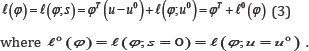
where y=(y1,.......,yn)T and u=u(y)=(u1(y),.....,uk(y))T is a sufficient statistic. Denote u 0=u(y0)and s =u-u0 where y0 is an observed data point. Then (2) can be rewritten as
In many applications, the parameter of interest is only a subset of the original parameters. Therefore, let φ=(ψT, λT)T.where is a d-dimensional parameter of interest and λ is a (k-d) -dimensional nuisance parameter. Then the log-likelihood function in (3) can be rewritten as

It is well-known that the conditional density of S1 given S1 = S2 is also a natural exponential family model and it has the form

which depends only on the parameter of interest ψ . Hence, according to Lehmann & Romano [1], inference concerning ψ will be based on the exact expression of (5). However, in general, both k1(ψ)and h1 (s1, s 2) are rarely explicitly available. Thus asymptotic methods are employed to obtain inference concerning ψ
.Two commonly used asymptotic methods are based on the asymptotic distributions of the maximum likelihood estimator and the log-likelihood ratio statistic. Let be the overall maximum likelihood estimate, which is obtained by solving

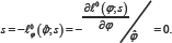
or, equivalently, by solving the score equation from (3)
Then, with the regularity conditions stated in DiCiccio et al.
[2],  is asymptotically distributed as a k-dimensional normal
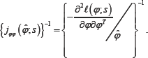
distribution with mean and variance-covariance matrix var ( )where var ( ) can be approximated by either the inverse of theFisher’s expected information matrix,
is asymptotically distributed as a k-dimensional normal
distribution with mean and variance-covariance matrix var ( )where var ( ) can be approximated by either the inverse of theFisher’s expected information matrix, 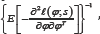 ,or the inverse of the observed information matrix
Since  is a (1Xd) vector of 1 and (1X(k-d)) vector of 0, we have is asymptotically distributed as a d-dimensional normal distribution with mean ψ and variance covariance matrix var
  ; or equivalently q
  isaasymptotically distributed as a chi-square distribution with d degrees of freedom, X 2d, Hence, the for testing
H0: ψ = ψ vs Hα:ψ ≠ ψo (6)
is approximately P (X2d>q(φ0)). Alternatively, let  be the constrained maximum likelihood estimate which can be obtained by solving

for each ψ Then, again with the regularity conditions stated in DiCiccio et al. [2], the log-likelihood ratio statistic
 2
2
is also asymptotically distributed as X2d. The corresponding p-value is approximately P(X2d >W(ψ0)).
The above two asymptotic methods are known to be not very accurate especially when the sample size is small [3]. In recent years, various higher-order asymptotic methods have been proposed to obtain more accurate results. In particular, the saddlepoint method discussed in Daniels [4] and some of the associated methods, have generated lots of discussions in statistics literature. Nevertheless, most of the researches in these higher-order asymptotic methods, such as the Lugannani and Rice formula, Lugannani & Rice [5], and the T* formula, Barndor-Nielsen [6,7], can only be applied to obtain inference for a scalar parameter of interest [8]. For a vector parameter of interest, only limited literature exists. For example, Skovgaard[9] derived a test statistic that was similar to the T* formula for a vector parameter of interest, and based on the idea from Fraser and Massam [10], Davision et al. [11] derived a directional test when the model is a linear exponential family model.
Note that the method by Skovgaard [9] attempts to correct the likelihood ratio statistic everywhere in the parameter space and, in general, is a relatively complicated method except for some special cases as those discussed in Skovgaard [9]. The proposed directional method, on the other hand, is designed to capture the alternative hypothesis suggested by the observed data. In Section 2, the directional test by Davison et al. [11] is discussed. It is then applied to testing homogeneity of the scalelike parameters of the inverse Gaussian distribution in Section 3. Numerical results are reported in Section 4 to demonstrate the accuracy of the proposed method. Some concluding remarks are recorded in Section 5 [12]
Main result
Fraser & Massam [13] derived a directional test as an alternate way for testing a vector parameter of interest. In the context of marginal inference for regression parameters in nonnormal linear models, this test avoids the computation for the high-dimensional marginal density by replacing them with a one-dimensional conditional density. In this section, we applied the methodology to the natural exponential family model with a subset of the canonical parameter being the parameter of interest.
For a natural exponential family model with canonical parameter φ=(ψT,λT)Tas discussed in Section 1, inference concerning will be based on the conditional density given in (5), which, in general, will not be explicitly available. Skovgaard [14] proposed a double saddlepoint method to approximate(5)On the other hand, Fraser et al. [12] proposed a sequential saddlepoint method to approximate the conditional likelihood function for and, hence, by normalizing the conditional likelihood function, we have

where c is the normalizing constant, Lo is a d-dimensional plane defined by s2 =0, is the overall maximum likelihood estimate of φ ψ is the constrained maximum likelihood estimate of φ for a fixed ψ and  is the determinant of the observed information matrix evaluated at the overall maximum likelihood estimate. Note that (7) is an approximation of (5) with the conditioning being implicitly accomodated by taking a "slice" through the full density. In other words, we are taking the full density but constraining s to lie s when
 be L+. Note that

and, thus, in (7) varies with s(t). As t increases, it traces a curve in the parameter space that passes through  In particular, when t = 0, it passes through and when t = 1, it passes through 0. Hence, by explicitly indicating that varies with S(t), the saddlepoint approximation of (7) constrained to L+ can be written as

To measure departure from the null hypothesis given in
(6) along L+ , we can use the conditional distribution of  given the unit vector
  this joint density of
  can be obtained by change of variable from s to .Then the marginal density of a can be obtained from integration and hence the conditional density is available. The most difficult part of the calculation is to obtain the Jacobian of the transformation. However, in Fraser & Massam [10], they have calculated the Jacobian to be proportional to td-1. Therefore,

As in Fraser & Massam [10], the p-value for testing the hypothesis in (6) can be viewed as the probability that S(t) is as far or farther from Sψthan the observed value 0. This p-value is referred to as the directed p-value, and mathematically, it can be calculated by
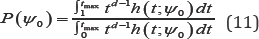
where tmax is the is the largest value of t for which the maximum likelihood estimator corresponding to .s(t) exists.
Application to testing homogeneity of inverse Gaussian scale-like parameters
The two-parameter inverse Gaussian distribution, IG ( μ,λ) has density
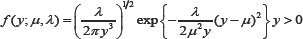
where μ>0 is the mean parameter and λ>0 is a scale-like parameter. Note that the IG (μ,λ) distribution belongs to the exponential family model with canonical parameters  This distribution is widely used to model positive right-skewed data. Doksum & Hoyland [15], Seshadri [16,17] and Takagi et al. [18] discussed applications of this distribution in accelerated life testing model analysis, survival data analysis and in occupational hygiene data analysis, respectively. Chhikara & Folks [19] examined the equality of means problem from k samples of independent IG(μi,λj) distributions, where i = 1,........,k. With the assumption that the scale-like parameters are the same, they derived the ANOVA F-test. Hence, testing

is of special interest. For testing the above hypothesis, Chhikara & Folks [19] and also Chang et al. [20] discussed the likelihood ratio test, and Wong [21] proposed a saddlepoint approach. For the rest of this section, the directional test approach discussed in Section 2 is applied to this problem.Let Yi1,....Yini be ni independent random variables from IG(μi,λj) distribution for i = 1,........,k. Moreover, assume these k inverse Gaussian distributions are independently distributed. Hence, the log-likelihood function is
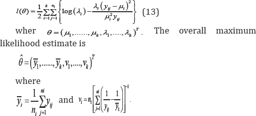
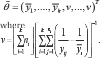
Further more, under the null hypothesis stated in (12) that the scale-like parameters are identical, the constrained maximum likelihood estimate is
Note that the model belongs to the exponential family model with canonical parameter φ=(φ1...φ2k)T
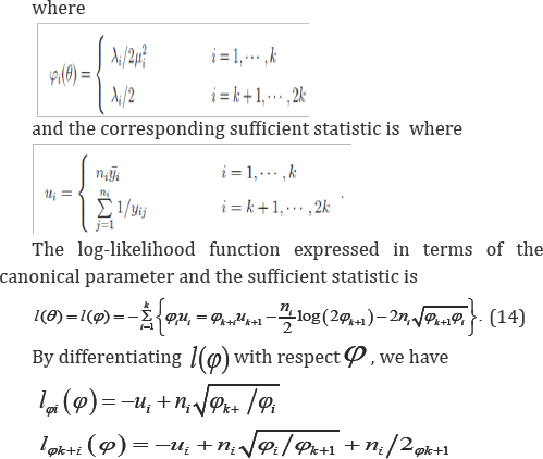
for i=1,.....,k Hence,the overall maximum likelihood estimate and the constrained maximum likelihood estimate of the canonical parameter are
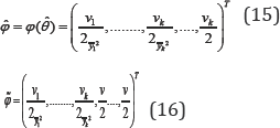
respectively. Moreover, let ψ=( ψ1,...., ψk-1)T where ψi=φk+1+i- ψk+i Then the hypothesis stated in (12) for testing homogeneity of the scale-like parameters can be expressed in terms of ψ by
H0: ψ= 0 vs Ha: ψ ≠ 0 (17)
Following the notation in Section 2, we have ψ0=0 , and
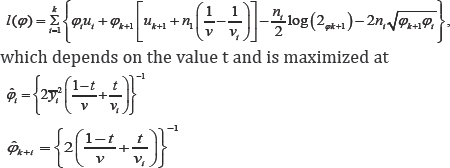
for i = 1,.....k. it is easy to show me when that t=0 and t=1, the maximize gives (16) and (15) respectively. Moreover, denote  where V(n)= max(V1,....,vn) is the largest value oft which the maximum likelihood estimator corresponding to s(t), exists. thus, by substituting all the necessary terms into (9) and we have
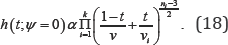
Finally, the directional p-value for testing homogeneity of the scale-like parameters can be computed from (11) with h(t) being defined in (18). Although there is no closed form for the integral, it requires only a one dimensional integral. Therefore,numerically, it can be easily obtained by some standard numerical integration routines such as those given in Maple, Matlab and R.
Numerical examples
In this section, we will first examine a real-life data example discussed in Kumagai & Matsunaga [22], which is a time series data set of chlorobenzene exposure concentrations (15 min TWAs) for a chemical worker (\Worker F" in the original paper) during a full workshift. The q-q plot in Takagi et al. [18] indicated that the (μ,λ) plot bin Takagi et al. [18] indicated that the IG (μ,λ) model is a reasonable model for analyzing this data set. Chang et al. [20] partitioned the data into the morning data and the afternoon data: (Table ) and assumed that the morning data and the afternoon data are samples from two independent IG(μ1,λ1) and IG(μ2,λ2) distributions. Table 1 records the p-values obtained for testing

H0 : λ1 = λ2 vs Ha : λ1≠ λ2
from the likelihood ratio method (lr) discussed in Chang et al. [20] , the Lugannani & Rice method [5] (LR) and the Barndorff- Nielsen[6] modified signed likelihood ratio method (BN)
discussed in Wong [21]and the directional method (Proposed) discussed in the paper. (Table 1)
H0 : λ1 = λ2
The methods discussed in Wong [21] have theoretical accuracy of O (n-3/2) The proposed
directional method give very similar result to that obtained by the Luggannani & Rice method [5]. Result from likelihood ratio method, which has theoretical accuracy of is not o (n-1/2) as close.
To compare the accuracy of the four methods, simulation studies were carried out. Following the set up in Chang et al. (2012), 5,000 samples are simulated for each settingS (n1,.....,nk) and(μ1,.....,μk;λ1,....,λk) With (λ1=.....=λk=λ As in Chang et al. [19],μ1,....,μkare all assumed to be 1. For each for each simulated sample, we compute the p-values using lr, LR, BN and Proposed methods. The simulated Type I error probability is the proportion of p-values less than the nominal significance level, which is chosen to be 0.05 and 0.1 respectively. The results are recorded in Table 2. It is clear that the lr method does not give satisfactory results unless n1,....,nk are large and the other three methods, regardless of the values of n1,....,nk give very similar type I error probabilities and they are close to the nominal significance level. More simulations with different parameter settings have been performed with the same pattern of results. They are not reported here, but are available on request.

Discussion
A directional test for a vector parameter of interest from a natural exponential family model is derived based on the likelihood-based higher order asymptotic methods. The p-value for the test required only a one-dimensional integration. The proposed method is then applied to obtain p-value for testing homogeneity of inverse Gaussian scale-like parameters. Numerical results indicated that the proposed methods are as accurate as the Lugannani and Rice method and the Barndor- Nielsen method, which are third-order asymptotic methods.
References
- Lehmann EL, Romano JP (2005) Testing Statistical Hypotheses. Springer New York, USA.
- DiCiccio TJ, Field CA, Fraser DAS (1990) Approximations of marginal tail probabilities and inference for scalar parameters. Biometrika 77: 77-95.
- Reid N (1996) Likelihood and higher-order approximations to tail areas: a review and annotated bibliography. Canadian Journal of Statistics 24(2): 141-166.
- Daniels HE (1954) Saddlepoint approximation in statistics. Ann Math Stat 25: 631-650.
- Lugannani, R. and Rice, S., 1980. Saddlepoint approximation for the distribution of the sum of independent random variables. Adv in Appl Probab 12: 475-490.
- Barndor -Nielsen, O.E., 1986. Inference on full or partial parameters based on the stan-dardized signed log likelihood ratio. Biometrika 73: 307-322.
- Barndor (1991) Modified signed log likelihood ratio. Biometrika 78: 557-561.
- Brazzale AR, Davison AC, Reid N(2007) Applied Asymptotics. Cambridge: Cam-bridge University Press, USA.this work is licensed under CreativeCommons Attribution 4.0 Licens DOI: 10.19080/BB0AJ.2017.03.555608
- Skovgaard IM (2001) Likelihood asymptotics. Scandinavian Journal of Statistics 28: 3-32.
- 10. Fraser DAS, Massam H (1985) Conical tests: observed level of significance and confidence regions. Statistics Hefte 26(1): 1-17.
- Davison AC (1988) Approximate conditional inference in generalized linear models. Journal of the Royal Statistical Society B 50: 445-461.
- Davison AC, Fraser DAS, Reid N, Sartori N (2014) Accurate directional inference for vector parameters in linear exponential families. Journal of the American Statistical Association 109: 302-314.
- Fraser DAS, Reid N, Wong A (1991) Exponential linear models: a two pass procedure for saddle point approximation. Journal of the Royal Statistical Society B 53: 483-492.
- Skovgaard IM (1987) Saddlepoint expansions for conditional distributions. Journal of Applied Probability, 875-887.
- Doksum KA, Hoyland A (1992) Models for variable-stress accelerated life testing experiments based on Wiener processes and the inverse Gaussian. Technometrics 34: 74-82.
- Seshadri V (1993) The Inverse Gaussian Distribution: A Case Study in Exponential Families. Claredon Press, Oxford.
- Seshadri V (1999) The Inverse Gaussian Distribution: Statistical Theory and Applications. Springer, New York, USA.
- Takagi K, Kumagai S, Matsunaga I, Kusaka Y (1997) Application of inverse Gaussian distribution to occupational exposure data. Annals of Occupational Hygiene 41: 505-514.
- Chhikara, R.S. and Folks, J.L., 1989. The Inverse Gaussian Distribution. Marcel Dekker, New York.
- Chang M, You X, Wen M (2012) Testing the homogeneity of inverse Gaussian scale-like parameters. Stat. Probab Lett 82: 1755-1760.
- Wong A (2016) Testing homogeneity of inverse Gaussian scale-like parameters: a saddlepoint approach. Statistical Papers 57(2): 319-327.
- Kumagai S, Matsunaga I (1995) Changes in the distribution of shortterm exposure concentration with different averaging times. Am Ind Hyg Assoc J 56(1): 24-31.


