


Consistency of the Semi-Parametric MLE under the Piecewise Proportional Hazards Models with Interval-Censored Data
Qiqing Y1* and Diao Q2
Department of Mathematical Sciences, SUNY, USA
Submission: August 24, 2017; Published: October 02, 2017
*Corresponding author: Qiqing Y, Department of Mathematical Sciences, SUNY, USA, Email: qyu@math.binghamton.edu
How to cite this article: Qiqing Y, Diao Q. Consistency of the Semi-Parametric MLE under the Piecewise Proportional Hazards Models with Interval-Censored Data. Biostat Biometrics Open Acc J. 2017; 3(2): 555606. DOI: 10.19080/BBOAJ.2017.03.555606
Abstract
We consider the piecewise proportional hazards (PWPH) model with interval censored (IC) relapse times under the distribution-free set-up. The partial likelihood approach is not applicable for IC data, and the generalized likelihood approach is studied by Wong et al. [1]. It turns out that under the PWPH model with IC data, the semi-parametric MLE(SMLE) of the covariate effect under the standard generalized likelihood may not be unique and may not be consistent. In fact, the parameter under the PWPH model with IC data is not identifiable unless the Identifiability assumption is imposed. They proposed a modification to the likelihood function so that its SMLE is unique. Under certain regularity conditions, we show that the SMLE is consistent and is asymptotically normally distributed.
Keywords: Coxs model; Time-dependent covariates; Semi-parametric MLE; Identifiability; consistency; Asymptotic normality
Abbreviations : PWPH: Piecewise Proportional Hazards; IC: Interval-Censored; PH: Proportional Hazards; TIPH: Time-Independent Covariate PH
Introduction
We establish the consistency of the semi-parametric MLE under the piecewise proportional hazards (PWPH) model, with interval-censored (IC) continuous survival time Y. The proportional hazards (PH) model specifies that a covariate vector Z has a proportional effect on the hazard function of Y. It is a common regression model for survival analysis. The PWPH model is a special PH model.
For a random variable Y, denote its survival function by SY(t) =P(Y > t), its density function by fY(t), and its hazard function by  Given a covariate (vector) Z which does not depend on time Y,(Z,Y) follows a time-independent covariate PH (TIPH) model or Cox's regression model if the conditional hazard function of Y | Z is

where βZ = β' z, β is the transpose of the vector β,τ = sup {t: ho (t)> 0} , and ho is an unknown baseline hazard function.
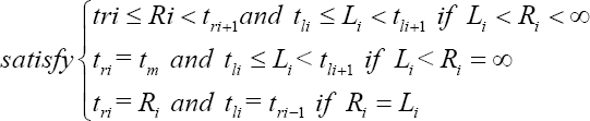
IC data consist of n time intervals with the end-points Li ≤ Ri,i = l,..., n , where the true survival time Yi falls inside the interval. Notice that (Li,Ri) is called left-censored if Li = -∞ right- censored if Ri=∞ strictly interval-censored if 0<Li< Ri< and exact if Li=Ri . Schick & Yu [2] proposed the mixed case interval censorship model to specify the IC data without exact observations as follows. Let K be the number of follow-up time for a patient. Conditional on K = k,Y and (Ck,1,.... Ck,k) are independent, where Ck,1...., Ck,k are the k follow-up times. The observable random vector is  ,where Ck,0 = 0 and Ck,k+1 =∞ . If P (K = m) = 1, then the mixed case model becomes the case m interval censorship model [3]. For Cox model with IC data, we assume that Z and (Y,K,C) are independent, where C = {Cki :i ∈{1,....., k}, k ≥ 1} .
The Cox model has been extended to the time-dependent covariates proportional hazards (TDPH) model. Cox & Oak [4] give a typical example of time dependent covariate in medical research, namely,

and c is the admission time to a treatment for a patient. They also give another example of time-dependent covariate. The TDPH model has been commonly used for right-censored (RC) data (see, for instance, Therneau & Grambsch [5], Platt et al. [6], Stephan & Michael [7], Masaaki & Masato [8], and Leffondre et al. [9]).
Zhou formulates a PWPH model with k cut points:

z =(z0, z1 ..., zk) is a time-independent covariate vector. Model (1.2) is a special case of the PWPH model (1.3) with a single cut point at c [10]. Wong et al. [11] applied the PWPH model to analyze their cancer research data. In a cancer research data set, Yi is the relapse time of a cancer patient after surgery, Zi is a vector with numerical or categorical coordinates, containing information about the age, tumor size at surgery, nodal number, bone marrow micro metastasis (bmm) or other information about the i-th patient. One is interested in the conditional survival function SY | z instead of SY. For instance, Wong et al. [11] considered a problem of studying the relation between the covariate bmm with IC relapse time Y of a breast cancer patient after the surgery. The covariate bmm is a categorical variable taking two values, say 1 (bmm positive) and 0 (otherwise). Some medical doctors suspected that the bmm effect might depend on time T. Then a PWPH model is as follows.
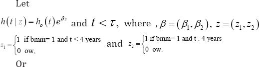
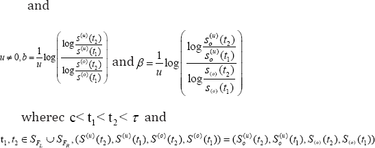
more z1= u1(t<c) general and z2= v1(t ≥ c), where a is a fixed constant, u and v are time-independent covariate vectors.
Under the TDPH model with RC data, a common approach is the partial likelihood approach. However, if the data is interval censored, even with the time-independent covariates, this approach does not work, thus Finkelstein [12] proposes the generalized likelihood function approach, making use of the generalized likelihood. Let So be the baseline survival function corresponding to ho and S (t | z) be the conditional survival function corresponding to h (t|z) in (1.1). Given IC data (Li,Ri,zi) which may contain exact observations, the generalized likelihood is

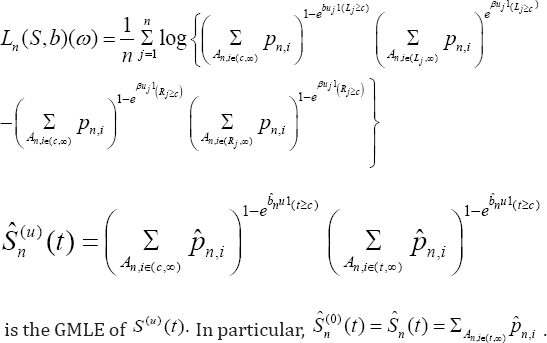
where δi = 1(Li = Ri) and S0(.) = S(.| 0) . The semi-parametric maximum likelihood estimator (SMLE) of (β,s0 ) , denoted by  , maximizes L over all survival functions So and all possible values of β.L defined in (1.4) is applicable to all IC data.
The semi-parametric problem under the PWPH model with IC data was studied by Wong et al. [1]. It turns out that under PWPH model(1) with IC data, the parameter β is not identifiable unless further assumptions are imposed (see Example 1). Moreover, in general, the SMLE of β under the likelihood function (1.4) may not be unique. Both phenomena do not occur if the covariates are time-independent . They specified the Identifiability condition for such problems and studied the estimation problem of deriving the SMLE. Their simulation results suggest that the SMLEs of So and β are consistent under the mixed case IC model [2]. We give the proof of the consistency and asymptotic normality of the SMLE in this paper.
The Main Results
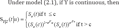
We study consistency of the SMLE under the PWPH model with one cut point assuming Y is continuous in this paper. In particular, we consider the model 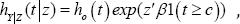 , where Z is a time-independent covariate vector (2.1). Y is subject to interval censoring under the mixed case IC model with the following up times Cki and the random number of follow-up times K. We first present some preliminary results [13].
Abusing notations, we write  . Without loss of generality (WLOG), we can assume that the covariates Zi, ∈ Rp and take at least p linearly independent values.
Given a random variable, say Y , let SFY be the support set of FY, in the sense that if x ∈ SFY then . SFL and SFR are defined in a similar manner.
Lemma 1: Assume the PH model  , with the parameter (β,So) and without censoring. Then the parameter (β,So) is identifiable, provided τ > C that , where
 .png) .
.
Lemma 2: Assume  . Under the mixed case IC model and assuming that S0 is absolutely continuous, the parameter β is identifiable if

The parameter So (c) is identifiable if β ≠ 0 in addition to assumption (2.2). If assumption (2.2) is violated, β is not identifiable, as is the case in the next example.
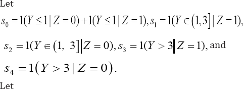
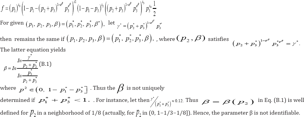
I. Example 1. Assume  . Let z ~bin(1,0.5) . Suppose that So ∈(0, 1)on (0, 4) . Moreover, assume the Case 2 model, that is, the observable random vector is
  where the censoring vector (u, v ) ≡ (1, 3) and So be absolutely continuous, where

Then is not identifiable. The proof is given in the Appendix.
The likelihood function with IC data is given by (1.4), i.e., . For the PH model, there are two differences between right censoring and interval censoring:
(a) One can show that the SMLE is unique and is consistent under the standard RC model but may not be so under the standard interval censorship model, unless further assumptions are imposed (due to Identifiability).
(b) The SMLE of So assigns weight to the cut point c under the IC model, but not under the RC model unless there exists an exact observation at c.
Let A1,..., Am be all the innermost intervals induced by Ii's . If the covariates are time independent, it is well known that in order to maximize L, it suffices to put the weights of So to the right-end points of the IIs. Let tj's be the right-end point of the II's, or c, or±∞ , t0=-∞<t1<......<tic =c< tic+1<...
The Theorem 1
Suppose that 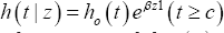 h, Y is continuous and subject to the mixed case IC model, E(k)∞ , and the identifiable condition in Lemma 2 is satisfied. Then the SMLE of is consistent.
Proof. We shall give the proof in 4 steps. Abusing notation, write be the sample space.
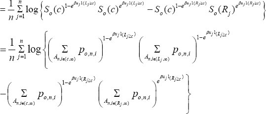
Step 1: (preliminary). Under the mixed interval censhorship model, by (1.4), the normalized generalized log-likelihood becomes Ln (S, b)
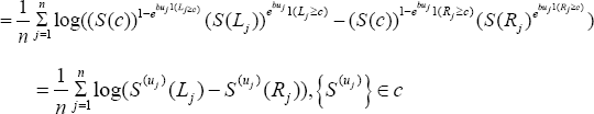
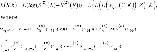
where C is the collection of all nonincreasing functions S from [0,∞;) into [0, 1] with S ( 0 ) = 1 and S (∞) = 0 . By the strong law of large numbers (SLLN), Ln (S,b) converges almost surely to its mean
Step 2: It can be verified that ws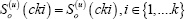 . Since sup{|plog p| : 0 ≤ p ≤ 1} ≤ 1, wS(u)(C,K) is bounded by K + 1, and thus L(S, b) is finite, as E(K) < ∞ by the assumption in the theorem. If the identifiable conditions hold, by Lemma 2 and the Shannon-Kolmogorov inequality, we can conclude that
  . As a consequence, for some
Thus b = β . Consequently, (So,β) maximizesL(S,b) and any other nonincreasing function s ͟ C and b satisfying L (S,b) = L(S0,β) satisfy S = So a.s.μ (the measure induces by dFL+dFR) and b = β .
 a.s let
  by the SLLN. Hereafter, we fix an w ϵ Ω0 and suppress it in the expressions of most random variables. For n > 0 , let Bn(®) be the collection of all the distinct points 0,Li,Ri,c, where 1 ≤ i ≤ n .Write Bn = {qn,j:1≤mn} , where 0 = q0 qn,1 <....< qn,mn = ∞
. Denote the intervals An,j= (qn,j-1, qn,j], 1 ≤ j ≤ mn . For each j, let p0,n,J = So(qn,j-1)-So(qn,j). Then
by the SLLN. Hereafter, we fix an w ϵ Ω0 and suppress it in the expressions of most random variables. For n > 0 , let Bn(®) be the collection of all the distinct points 0,Li,Ri,c, where 1 ≤ i ≤ n .Write Bn = {qn,j:1≤mn} , where 0 = q0 qn,1 <....< qn,mn = ∞
. Denote the intervals An,j= (qn,j-1, qn,j], 1 ≤ j ≤ mn . For each j, let p0,n,J = So(qn,j-1)-So(qn,j). Then  for each t∈Bn. Moreover, the normalized log-likelihood function with s = So is Ln (So, β) (ω)
Now we assign weight pn,i to each interval An,i with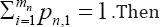 .Then
.Then
Let {Sn (x)} be a sequence in C By a point wise limit of this sequence we mean S* ∈ c such that Sn, (x) → S* (x) for all
x and some sequence {n'}n'≥1 . Let s(0)* (t) be the point wise limit function of  for all t and for some subsequence {n'}n'≥1 . Helly's selection theorem guarantees the existence of point wise limits. Let b* be the limiting point of
 for some subsequence {n"}n''≥1 of {n'} .
Since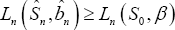 by the definition of the GMLE, the claim in Step 3 is proved.
Step 4 (Conclusion). Let  denote the empirical estimator of Q the distribution of (L,R,Z) and
 a.s. for every Borel subset
 survival function defined by
 . For simplicity in notation we shall assume that Sn (x) — S* (x) for all x ∈ R and bn — b*


By the previous discussion, it suffices to prove the last inequality.
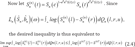
which follows from Lemma 3. It follows from inequality (2.3) that L (S*, b*)≥ L (So ,β) . As (So ,β) maximizes L, we can conclude that L (S*, b*) = L (So, β) and therefore S* = So, a.s. μ . If the identifiable conditions (2.2) holds, we have b* = β .
Lemma 3. Inequality (2.4) holds.
In order to prove the Lemma 3, we will introduce the Fatou's Lemma with varying measures.
Theorem 2.
Suppose that μn is a sequence of measures on the measurable space (S, Σ) such that μn (B ) — μ(B), ∀B ∈Σ . Then, with fn non-negative integrable functions and f = lim infn—∞ fn. Then
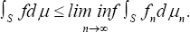
Proof of Theorem 2: We will prove something a bit stronger here. Namely, we will allow fn to converge μ-almost everywhere on a subset B of S. We seek to show that  .
.
 Thus, replacing B by B \ K we may assume that fn converge to f pointwise on B.
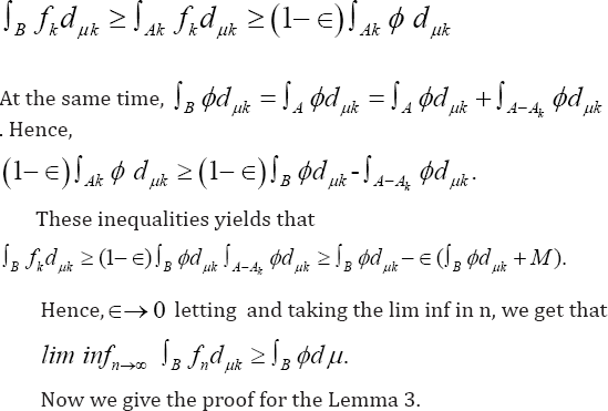
Recall that a simple function ø is of the form that  where Ai's are disjoint measurable sets. Given a simple function ø we have
  . Hence, by the definition of the Lebesgue Integral, it is enough to show that if is any nonnegative simple function less than or equal to f, then
Let a be the minimum non-negative value of ø . Define A = {x ∈ B :ø(x)> a} . We first consider the case when ∫Bø dμ =∞ We must have that μ (A) is infinite since ∫Bødμ≥M μ( A), where M is the (necessarily finite) maximum value of that ø attains. Next, we define  But An is a nested increasing sequence of functions
At the same time,  proving the claim in this case ∫B ødμ< <∞;. It suffices to prove the theorem in the case . We must have that μ( A) is finite. Denote, as above, by M the maximum value of (ø) and fix ∈> 0 . Define
  . Then An is a nested increasing sequence of sets whose union contains.
Thus, A - An is a decreasing sequence of sets with empty intersection. Since A has finite measure (this is why we needed to consider the two separate cases), llmn→∞μ( A — An ) = 0. Thus, there exists n such that 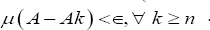 since
since 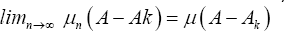 , there exists N such that
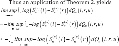
Proof of Lemma 3 Since and
and  for evrey
  .
.
Theorem 3
Suppose that the assumptions in Theorem 1 holds and the support set  contains finitely many elements. Then the SMLE of (So, β) is asymptotically normally distributed.
Proof: By assumption  and m is finite. Then the parameter (So,β) can be represented by (So (t0), ..., S(tm), β), and the problem becomes an estimation problem of a multinomial distribution subject to certain constraints. Thus the asymptotic normality follows and the asymptotic covariace matrix can be estimated by the inverse of the empirical Fisher information matrix.
 realization. The joint density is
References
- Wong GYC, Diao QG and Yu QQ (2017). Piece-wise Cox Models with interval censored data.
- Schick A, Yu QQ (2000) Consistency of the GMLE with mixed case interval-censored data. Scand J Statist 27(1): 45-55.
- Groeneboom P and Wellner JA (1992) Information bounds and nonparametric maximum likelihood estimation. Birkh a user Verlag, Basel.
- Cox DR and Oakes D (1984) Analysis of Survival Data. Chapman & Hall NY.
- Therneau T, Grambsch P (2000) Modeling survival data: extending the Cox model. Springer.
- Platt RW, Joseph KS, Ananth CV, Grondines J, Abrahamowicz M, et al. (2004) A proportional hazards model with time-dependent covariates and timevarying effects for analysis of fetal and infant death. Am J Epidemiol 160(3): 199-206.
- Stephan L, Michael S (2007) Parsimonious analysis of time-dependent effects in the Cox model. Statistics in Medicine 26(13): 2686-2698.
- Masaaki T, Masato S (2009) Analysis of survival data having time- dependent covariates. IEEE Trans Neural Netw 20(3): 389-394.
- Leffondre K, Wynant W, Cao Z (2010) A weighted Cox model for modeling time-dependent exposures in the analysis of case-control studies. Stat Med 29(7-8): 839-850.
- Zhou M (2001) Understanding the Cox regression models with timechange covariates. American Statistian 55(2): 153-155.
- Wong GYC, Osborne MP, Diao QG, and Yu QQ (2016) Piece-wise Cox Models with right-censored data. Comm. Statist Comput Simul.
- Finkelstein DM (1986) A proportional hazards model for interval- censored failure time data. Biometrics 42(4): 845-854.
- Wong GYC, Yu QQ (2012) Estimation under the Lehmann regression model with interval-censored data. Comm Statist Comput Simul 41(8): 1489-1500.


