Review Article

A New Method of Clusters Definition Based on a Saccadic Model of Human Vision

Roman Tankelevich*

California State University, USA, Computer Science Departments at Long Beach and Dominguez Hills, CA

Submission: December 20, 2023; Published: February 14, 2023

*Corresponding author: Roman Tankelevich, California State University, USA, Computer Science Departments at Long Beach and Dominguez Hills, CA

How to cite this article: Roman Tankelevich. A New Method of Clusters Definition Based on a Saccadic Model of Human Vision. Ann Rev Resear. 2023; 8(3): 555739. DOI: 10.19080/ARR.2023.08.555739

Abstract

In [1], the inverse problem related to the EEG based test of the brain’s electrical activity was scrutinized. The analysis had suggested that the measured EEG potentials are caused by the sets of activated neurons – the clusters whose locations can be found by using a Deep Learning Neural Networks. Here, we present a method to extract the features/shapes of the clusters used in classification. The suggested Boundary Function Method (BFM) employs the following approach. A cluster as a subject of classification is inscribed into a regular region such as a circle (a sphere) and the projection of the clusters’ image onto the region’s boundary is produced and analyzed as a boundary function. Different methods of such mapping of the image onto the boundary are considered. Among them are the methods of Fundamental solutions of the Laplace equations, Radial Base functions, Gaussian models, and others. The boundary functions are analyzed to extract the cluster’s features. The extraction of the features is performed by FFT, wavelet analysis, and other analytical methods applied to the boundary function. The extracted features are used in the classification performed by various methods, such as KNN, SVM, CNN, LSTM and other learning techniques including the Deep Learning methods. The Boundary Function Method was used in experimental analysis of both regular and irregular shapes of the clusters. The method was also applied in the context of a real-time image processing including segmentation and object identification based on a saccadic model of human vision – the tasks related to the self- driving and self-controlled driving machines, robotics, and other automatic control systems. Finally, the BFM was tested by using some real-life datasets such as the one for the lung X-rays related to Covid-19.

Keywords: EEG; Inverse problem; Neuron clusters; MFS; FFT; RBF; Wavelet analysis; Covid-19; Feature extraction and classification

Abbreviations: CNN: Convolutional Neural Networks; GPU: Graphics Processing Units; DETR: Detection Transformer; BFM: Boundary Function Method; FFT: Fast Fourier Transform; COI: Cluster of Interest; MSER: Maximally Stable Extremal Regions; LSTM: Long Short Term Memory

Introduction

In [1], a case of the inverse problem solution was applied to the EEG imaging. It was shown that the solution can be presented as a set of clusters of electrical sources. In this paper, we propose a method of extracting the information about the shape of the clusters based on their mapping onto the encompassing boundary.

In the context of the EEG imaging and beyond it, the following tasks are considered here:

Medical Imaging

i. Given is a Euclidian domain G with a finite set of points (neuron locations) assigned the binary values 0-1. The locations ascribed 1 represent the identified sources in the EEG problem. The sources are assumed to be located compactly, by forming the clusters obtained as a solution of the inverse EEG problem. In the 2D settings, the task is to detect and identify the patterns in the pixelated black-white images. The task is to identify and classify the found clusters.

ii. The same task but related to the clusters of real valued sourc es such as those presented at the fMRI and CT- Scan imaging.

Pattern Recognition in Technical Field

a. The task of finding and classifying the objects inside the bitmapped images collected from image capturing devices.

b. Image and pattern recognition, specifically in relation to the self-driving and self-controlled driving machines, robotics and other automatic control systems.

In this paper, we discuss a novel approach, the Boundary Function Method, as a technique applicable to the above tasks and providing, presumably, their effective solution. Among many recently published techniques and methods, we can mention here, as a counterpart of the BFM, such methods as R-CNN, Fast R-CNN, R-CNN and YOLO of different versions (most recently, YOLO v.4) [2-5]. In one group of such methods, the object detection is performed by repurposing classifiers from detection to classification. The use of object proposals is an effective recent approach for increasing the computational efficiency of object detection. A novel method for generating object bounding box proposals using edges was suggested independently. Edges provide a sparse yet informative representation of an image. Main observation is that the number of contours that are wholly contained in a bounding box is indicative of the likelihood of the box containing an object. The major advantage of the methods belonging to the YOLO group, on the other hand, is that a single convolutional neural network is used simultaneously for finding the bounding boxes and for identifying the objects inside them. The Convolutional Neural Networks (CNN) are trained for full images and can outperform many other methods of the image recognition and classification. Most of the CNN-based object detectors are largely applicable only for recommendation systems. Improving the real-time object detector accuracy enables using them not only for hint generating recommendation systems, but also for stand-alone process management and human input reduction. Real-time object detector operation on conventional Graphics Processing Units (GPU) allows their mass usage at an affordable price. The most accurate modern neural networks do not operate in real time and require large number of GPUs for training with a large mini-batch-size. The effort was made to create a CNN that operates in real-time on a conventional GPU, and for which training requires only one conventional GPU.

One of the latest developments in image detection is a new framework, Detection Transformer (DETR), developed at Facebook AI. Its purpose is to serve as a unified platform that generalizes sufficiently well using limited number of parameters. DETR is provided with a small number of learned object queries. The outcome of DETR is a suggestion about how the objects relate to the global image context. As a result it outputs the set of predictions in parallel. The core of the technology is the ideas of Transformer and the concept of Attention popularized within the areas of Natural Languages Processing and the technique called LSTM (Long Short-Term Memory) [11-12,14]. Recently, a method of Panoptic segmentation that unifies the typically distinct tasks of semantic segmentation (assign a class label to each pixel) and instance segmentation was considered [13]. All these approaches and methods have been successfully used in the tasks of parsing and recognition of regular patterns. However, they are not suitable to the task of the clusters classification as it appears in the context of the indirect reconstruction of the images. That is because the shape of a cluster of activated neurons cannot be accurately recognized if only the boundary conditions for the whole set of the clusters are given like in the case of the inverse problem concerning the EEG method. We pursue the task of finding a method that would be equally applicable to the regular images such as the ones found in the general image recognition arena as well as the bio-medical clusters recognition and identification. One of the significant properties of such a method should be its limited complexity. The Boundary Function Method (BFM) discussed here is based on the following approach: to identify the shape of an individual cluster, all its elements are mapped onto an artificial boundary around that specific cluster. An imaginary boundary function is estimated by mapping all the elements of the cluster onto this boundary. Then, the boundary function is subjected to analysis with the purpose to extract the cluster’s features. Such an analysis has a reduced complexity due to decreasing dimensionality of the task.

The Principles and Elements of the BFM

In the context of the EEG based bio-medical imaging, all the clusters are obtained as the result of analysis of the boundary potentials given by the EEG measurement. The BFM’s purpose is opposite: the clusters are given a priori, resulted, for example, from MRI, CT-scans or various computer vision means, while a single cluster is inscribed into an artificial boundary to which the cluster is mapped. The boundary function resulted from the mapping, is used to extract the features of this cluster, such as the parameters of the multifaceted image representation (number of faces and vertices); elements of the affine transformation, etc. Finally, the clusters are subjected to classification based on the information contained in the boundary function.

General review of the BFM

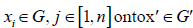
The suggested approach called here Boundary Function Method (BFM) leads to decreasing the dimensionality of the machine learning task by projecting a given N-dimensional image onto its N-1-dimensional boundary. (The same effect of reduced complexity is targeted by using the Convolutional Neural Networks which extracts the features of the image by applying the convolutional filters; however, the BFM seems to be more economical.) Here, we consider only two-dimensional clusters assuming that some of the results of this analysis can be applied to the similar multi-dimensional clusters, as well. The approach suggested here is also characterized with the way a single cluster is extracted from the overall image of multiple clusters. Only a part of the overall image is selected by being put “under a spotlight” using the method found in the saccadic movement characteristic for the human vision. Thus, the image inside the given domain G(x) under the spotlight is mapped onto the boundary 𝐺′(𝑥′). The mapping can be performed using any distance-based function. The resulted boundary function S(𝑥′) will be used for a feature extraction to characterize the cluster under the spotlight. The task of this report is to investigate the efficiency of the BFM and its ability to extract significant features of the selected clusters. The scope of this analysis includes both regular and irregular cluster images with the binary and real- number values of neurons’ states. The study of this method is performed here with the purpose of understanding how much the properties of the clusters can be exposed by mapping their elements on the artificially created boundary.

We also suggest that the Boundary Function Method can be applied, in addition to the biomedical images, to general pattern recognition tasks. The mapping of a pixelated image onto its boundary leads to a reduced dimensionality of the classification task and, as the result, can promote the increased speed of classification - one of the reasons to investigate the approach. Here we consider different methods of mapping the clusters onto the boundary – linear functions, radial base functions, Fundamental solutions of the Laplace operator (both 2D and 3D), etc. The feature extraction using the boundary function is analyzed by using different modalities: Fourier Transform (including Fast and Discrete Fourier Transforms), wavelets, etc. The methods of the analysis based on the use of the boundary functions were investigated in some works. We mention here two of them: In [9], the task of classification of 2D images is presented in terms of solution of a Poisson equation for the domain presented as the image to be identified with the boundary condition using the MFS method [7]. A 3D void detection using MFS [8], also, comes close to this subject.

Implementation details and propositions

The experiments with BFM were conducted within three areas of application: (a) identification of the regular geometric shapes; (b) detection and identification of the 2D images, and (3) the bio-medical imaging. A few computing platforms were used including MATLAB, Python, TensorFlow, Kaggle, Jupiter Notebooks, as well as the libraries such as Open CV. Proposed here model of detection of an object to be identified in an image is based on a saccadic mechanism similar to the human vision model. As applied to the image detection in the given 2D pixelated pictures, the human vision model is considered having such elements as saccadic search of objects in the picture; support of active and peripheral views; and detection of the image of interest followed by its classification based on the learning mechanism. In this work, the following propositions are used:

i. Proposition 1: In saccadic movements of the vision apparatus, the fixation points of vision are found based on the amount of “energy” produced by the image inside the saccade area.

ii. Proposition 2: The signal energy is mapped to the circumference of the vision field. It is performed by mapping the inside signals (pixels) by using different kernels (possibly, 2-D and 3-D fundamental solutions of Laplace operators, radial functions, Gaussian kernels, etc.)

iii. Proposition 3: The signal energy as calculated to the circumference can be subjected to the spectral analysis to extract the shape features – the information about the shape of the inscribed body with, optionally, parameters of affine transformation.

Method of calculating the field energy applied to the boundary

E = KΘPixels

where K is the mapping kernel, Pixels are the points values on the scan lines inside the vision field, and Θ is an operator of the mapping.

Algorithm of detection and selection – specific features

Given a 2-D pixelated Image 1.

These steps conclude the detection and analysis (possibly, general and non-specific) of the body of interest. If this is applied to the task of catch and follow algorithm, the saccadic search is stopped, and the vision field follows the found image.

Algorithm of classification

If the detection algorithm has produced an object of interest (with some general properties identified) it can be subjected to classification analysis by using one of the learning algorithms. More specifically, in this work, the algorithms of K-NN, SVM, LSTM, and Deep Learning ANN and CNN were tested.

Finding areas of significant “energy”

The algorithm of MSER (Maximally Stable Extremal Regions) implemented on different platforms including MATLAB was used to detect the stable regions of the image. The MSER detector incrementally steps through the intensity range of the input image to detect stable regions. The Threshold Delta parameter determines the number of increments the detector tests for stability.

regions = detectMSERFeatures(I)

returns an MSERRegionsobject, regions, containing information about MSER features detected in the 2-D grayscale input image, I.

[regions,cc] = detectMSERFeatures(I)

optionally returns MSER regions in a connected component structure.

[_]= detectMSERFeatures(I,Name,Value)

sets additional options specified by one or more Name, Value pair arguments.

Expected benefits

Using the boundary values instead of the original objects means reduction of dimensionality. This effect leads to the speeding up the detection and identification of the objects. The feature extraction (such as spectral properties by using FFT) reduces the number of classes. It becomes possible to create a hierarchy of classes (e.g., classes of all polygons of different arity). It also allows for geometrical and topological invariance (such as affine transformation). The following is presented in the paper. The cluster is inscribed into a regular region such as a circle (a sphere) and the projection of the clusters’ image onto the region’s boundary – the boundary function – is produced and analyzed. Different methods of such mapping of the image pixels onto the boundary (Fundamental solutions of the Laplace operator, Radial Base functions, Gaussian and others) are considered. The boundary functions, then, are analyzed to extract the cluster’s features. The extraction of the features is performed by FFT, wavelet analysis, and others. The extracted features are used in the classification. The method was subject to experimental analysis of the shapes. Also, it was assumed and analyzed as part of a segmentation and identification system based on a saccadic model of human vision. Finally, the method was tested by using some real-life datasets such as the one for the Covid-19 Lung X- rays. In Appendices 1 and 2, the experimental results are presented for clusters of regular and irregular shapes. In Appendix 3, we discuss the saccadic model of the image segmentation and identification that can be used in different image recognition environments.

Overview of the BFM

The algorithm is illustrated by Figure 1 as it applies to the analysis of the brain clusters. This flowchart presents the following data and control flow:

i. Scan (deterministically or randomly) over the view field; in the real time applications, this is analogous to the saccadic movements of the viewer’s eyes

ii. Identify the regions (circular) of potential interest based on the “energy” estimate collected on the region’s boundary

iii. Inscribe Cluster of Interest (COI); adjust COI using MSER in size (R) and position (the center point) to maximize the boundary energy under some constraints

iv. Calculate boundary function by using FFT, RBF, MFS, etc.

v. Produce Feature Extraction (the topology properties, shape - number of edges, affine parameters, etc.) by using FFT, convolutional centers, etc.

vi. Perform classification of the found subject by using the Deep Learning or other classifiers.

Operators Used for Mapping and Feature Extraction

Radial Base Function

By its definition, a radial base function (RBF),

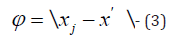
ψ (＼x − x0 ＼) for a point 𝐱 in the Euclidean space, is a real function that depends only on the distance from another fixed point, 𝐱0, called center. For a given domain 𝐺 and its boundary 𝐺′, consider a boundary function 𝑠(𝑥′) that maps the 𝑛 points

by using radial base functions

Ψ(＼.＼), namely by defining the boundary values 𝑠(𝑥′) for

𝑥′ ∈ 𝐺′ via the centers 𝑥𝑗 inside the given domain:

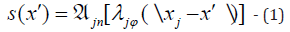
where is an aggregate operator such as

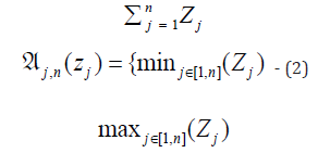
(Here 𝜆_𝑗 are scalars; most commonly 𝜆>_𝑗=1 for all 𝑗.)

In our consideration, the centers are taken as the points belonging to a given domain and representing pixels in the images, neurons in the EEG maps, and other elements of the original data.

Distance based functions

In the analysis described here, the following distance-based functions are considered.

a) Linear function

1.

2. as a partial case of polyharmonic splines

3.

b) Fundamental solutions of the Laplace equation

i. 2-dimensional case:

4.

ii. 3-dimensional case:

5.

c) Gaussian

6.

Feature extraction

Filters are applied to the boundary function 𝑠(𝑥′), in order to extract the features identified with use of harmonics.

Fourier Transform: This transform is used to extract harmonic members of the function. The frequencies with larger amplitudes characterize the images with specifically expressed polygonal shapes. The Fourier Transform can be used in both continuous and discrete forms. In the continuous case, the extracted frequency related features, 𝐟(𝜔), are calculated as follows:

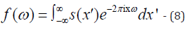
The FT is most efficiently performed as Fast Fourier Transform which is used in this research.

Short-Time Fourier Transform: The FFT was applied also to subsections of the given function 𝑠(𝑥′). This is performed with the STFT method that uses the sliding window applied to the sections of the input function. The method is supposed to extract harmonics from s(𝑥′) in assumption that it is a non-stationary function.

Wavelets: The wavelets provide a rigorous analysis of localized spectral properties of the boundary function. Applying the wavelets can provide some additional information.

Convolutional filters: More general approach can be considered as collocation,

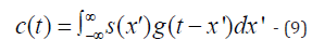
Here 𝑔(𝑦) is a collocational kernel. By applying it to different parts of the boundary function, the corresponding feature will be extracted as a function 𝐜(𝐭). This filter can be presented as a compactly supported function, thus providing a compact feature.

Experimental Results

We consider three areas of experiments concerning:

1. Regular Clusters

2. Clusters of irregular shapes in 2D pictures (e.g., as captured in automatic driving systems)

3. Irregular shapes in bio-medical images (including CT-scans and X-rays of lungs)

A. Regular Clusters

Experiments were conducted with clusters having the polygonal boundaries of different arity, size, position and regularity. The clusters were inscribed into a circular spot and the boundary function was calculated using different mapping methods as described in IV.A and IV.B. Then, the analysis of the boundary function was performed by applying different feature extraction methods described here.

I. Experiments: The objects of these classes can be resulted from some affine transformations of the given clusters, thus the finding of the object of a specific class should be complemented with information about its placement (e.g., the anchor information).

a) The general task

Given a 2D picture with a set of pixelated clusters P belonging to a set of predefined images C (objects), DETECT and IDENTIFY the classes to which the images belong to. The images of a specific class of geometric objects (triangles, pentagons, etc.) can be translated, rotated and scaled.

b) The task of identification of images of specific classes

The given image is placed into a specific Spotlight used for calculating the boundary conditions for the image. For simplicity sake, the boundary of the image is approximated as a polygon. Two cases of the Spotlight domain where the test clusters can be inscribed were considered originally:

i. Rectangular, and

ii. Circular domains

Further in this study, a circular Spotlight area with an image inside (clusterized pixels of assigned values/colors) is considered and used to identify the predefined classes of specific clusters of pixels.

c) The Method

The area of the given picture inscribed within the Spotlight boundary B(x,y) is populated with a set of random points, pr(x,y). The points belonging to a specific channel (more likely, colors of the objects to be detected) are used in calculating the functional, for example, the 2D Laplace Fundamental Solution Sum(1/r(pr, B(x,y)), where r() is the distance function. Thus, boundary points obtain the values the set of which characterizes the class and transformations of the object inside the domain. This set of points is a boundary function representing the inscribed object.

d) Preprocessing for classification:

The boundary function is preprocessed as needed. The preprocessing is used to extract the image features for its identification. For example, the Fast Fourier Transform (FFT) is performed to identify the periodic properties of the cluster boundary.

e) Training: A generative data set is used by creating different samples of the classes under consideration and calculating the boundary conditions by using the above functional.

B. Experiments with regular clusters identified by BFM

In the experiments with the regular images, the following approach was used.

All image pixels, 𝑝, are mapped onto the border, 𝑏. Different mapping function, 𝑓(𝑏), were considered including the Radial Base functions, such as f(b) = Σ∀p1/ r( p,b) .

The calculated boundary conditions are presented as a list of real values, 𝑉 = 𝑓(𝑏), associated with all selected points, 𝑏, on the boundary. All experiments were performed for a circular domain Ω=[C, R] defined with its center C and radius R. An inscribed cluster representing the image I is a set of binary values assigned to the nodes of the grid G imposed on Ω. The boundary condition list calculated at the preprocessing stage is used as an input of a feed forwarding ANN which output is the clusters likelihood and the classes they belong to. The ANN is to be pretrained on a set of generated data. Note: This approach is different of semantic segmentation methods which consider the whole image as an input. In the BFM, the assumption is that a one-dimensional input can be used for training and applying the model which should allow to expediate the solution (in terms of Frames-Per- Second metric used, for example, in image recognition within the automatic driving context). This research should answer the following questions: (1) is the boundary information sufficiently sensitive to recognize the cluster’s shape (class); (2) how trainable the model would be; (3) how many different clusters can be recognizable simultaneously.

C. Technique and Examples

a) A regular shape within a circular Spotlight

Consider a cluster shaped as a pentagon (Figure 2) Given the circular Spotlight Ω=[C, R] with its circumference, Boundary, and the array of random, uniformly distributed, pixels, Spotlight Points, (green colored and initialized with 0’s) inside it, a specific Spotlight function, SL, is calculated. In this example, a fundamental solution of the 3D Laplace Equation is used as the specific function. By definition, it is the matrix of reciprocals of the distances between the Spotlight internal points and the points on the boundary:

DM_data = Dist Matrix (Boundary, Spot Light_Points); SL = 1./ DM_data - (10)

A pentagon cluster inscribed into the Spotlight is a set of the cluster’s pixels

Cluster_Points ⊂ SpotLight_Points - (11)

as its subset (red pixels in Figure 2). The cluster’s pixels are ascribed the active status (value 1):

Active_Vector = ones (Cluster_Points); - (12) Thus, the boundary function is calculated by mapping the

Active_Vector onto the boundary by SL as a map:

Boundary_Function= SL*Active_Vector; - (13)

(Note that SL is specific for a selected spotlight and its mapping function, thus, needs to be calculated only once.). The Boundary_ Function is calculated for a given number of boundary points. Figure 3 shows the boundary function, BF(n), calculated in interval of points on the boundary n ∈ [1, N], N = 100. The function oscillates with 5 peaks corresponding to five faces of the inscribed pentagon. The relationship between the polygon’s shape and the oscillations in its boundary function was found in other regular shapes as shown in Figure 4. Examples of oscillating boundary function. The oscillation frequency Fr(BF) represents the number K of edges of regular convex clusters shown here: K=1 for a circle; K=3 for a triangle; K=4 for a square, etc. Oscillation frequency of the boundary function is used as a characteristic feature of the inscribed cluster to be recognized. The spectral analysis of the boundary condition provides information about periodic properties. The higher harmonic represents the number of edges; their phase information indicates the affine transformation parameters. The spectral analysis of BF is performed by using the Fast Fourier Transform, fft(), applied to an array of N (=100)discrete real values, and by calculating the spectral power ( fft()returns the Fourier coefficients):

ft = fft(BF, 100); - (14)

power = abs(ft).^2/100; - (15)

For regular shapes, the plotted power function, power(n), exhibits a peak at the X-value corresponding to the number of edges. Below, on Figure 5(a-d) an example of analysis for a loosely populated square cluster (a), its boundary function (b), the spectral power (c) and the Fourier coefficients (d) are presented. A rotated image has the same frequency characteristic as the original one. Its rotated position can be identified by the distribution of the Fourier coefficients (see Figure 6(a-d) (b) and (c)) as compared to Figure 5 (d). As seen from the examples above, the rotational transformation of the cluster can be identified by the coefficients excluding those close to 0. They are

(-6.0 ± 0.75i) in Figure 5d,

(6.0 ± 0.9i) in Figure 6b,

(-0.7 ± 6.0i) in Figure 6c.

The factor identifying the position of the body inside the Spotlight can be defined by the ratio of the real and imagery parts of the Fourier coefficients. Translation effect is illustrated by an example in Figure 7. Thus, the spectral power and Fourier coefficients are significant features of the regular clusters in the Spotlight as identified by the Boundary Function. They can be used in the training of the ANN to recognize the geometry of the regular clusters inside the Spot Light.

b) Other observations and conclusions

In Appendix 2, more examples of the analysis of regular clusters are presented. They concern various forms of the mapping used to create the boundary functions for the included object. Specifically, the following functions were considered: Fundamental solution functions of various PDE; Gaussian RBF, Min/Max mapping functions, and others. Also, the effect of saccadic movement in the capturing of an object to be analyzed is considered. As it was illustrated earlier, the boundary function calculated for the regular clusters exhibits oscillations. The number of peaks in the BF is roughly equal to the number of vertices in the polygonal cluster. By applying the Fourier transform (specifically, Fast Fourier Transform, FFT) this feature can be extracted from a periodic boundary function. By using the power function calculated as the result of the FFT, the periodic properties are exposed very clearly. The mean value of the BF reflects the size of the cluster; more specifically, the area occupied by the cluster as related to the area of the SpotLight.

If the cluster has a smooth boundary, without sharp edges, no oscillations are observed. It was also found that rotation and translation of a cluster can be exposed by analyzing the boundary function and its FFT. As the result of the affine transformations, the BF preserves the oscillating pattern but changes its regular shape, thus introducing some additional, higher harmonics. Also, the closer the cluster to the border, the lesser details are exposedeventually, the BF becomes the curve with just one peak. When scaled down, the curve becomes more “pronounced”. Most commonly, the task is to classify a cluster. It was found that the features that can be used to identify the type of the regular clusters are the most significant complex Fourier coefficients and the frequency of the harmonics.

The sensitivity of image recognition depends on the methods of the mapping of the cluster onto the boundary of the SpotLight. It was found that using the 3D fundamental solutions (1/r) of the Laplace equation provides higher boundary function sensitivity to the affine transformations than the corresponding 2D fundamental solution, ln(r). Some other RBF functions can be used efficiently, as well. For example, the Gaussian RBF with a zero mean value and a given standard deviation, sigma, was experimented with, as well. The mapping is characterized with the following specific Spotlight function using DM_data of (10):

SL = exp(-DM_data.* DM_data ./sigma); - (16)

In experiments with different regular clusters it produces the results similar to other mapping functions but more controllable by using sigma as a parameter. Most of the experiments here were provided for singly connected clusters (with no holes). Also, an algorithm was developed for analyzing the regions with thin borders – that is, essentially, the cases of multiply connected clusters with one large hole. The analysis of singly connected clusters using their thin borders would require less calculations in mapping the cluster’s pixels onto the boundary of the SpotLight. The scanning of a black-white images, in such cases, needs to follow the scan lines only until the pixel value has changed from 0 to 1 and vice versa. The Active_Vector in [12] becomes smaller, thus the computing Boundary_Function = SL*Active_Vector; as in [13], has 1D complexity instead of 2D. It was shown that this method of mapping provides the same identification features as in the analysis of the full body (Figure 8). Other investigated cases of mapping the pixels, Active_Vector, onto the SpotLight boundary were the ones based on using the MIN(R) and MAX(R) mapping functions. The specific function, SL, associates each point, P, on the Spotlight boundary with the points on the radius to P. The mapping of the cluster onto the boundary is based on finding the minimum/maximum distance of the cluster’s pixels to each point on the border It is a computationally efficient method. Its testing showed results very similar to other investigated methods concerning the convex regions. The MIN(R ) vs. MAX( R ) is preferable since it does not produce the additional harmonics in the boundary function (the MIN(R) produces a smoother boundary function) (Figure 9).

c) Capturing an object of saccadic search

As it was found in the experiments described above the sensitivity of the boundary function to the shape of the body inside the SpotLight depends on the body’s position. The body can be adjusted inside the circle as part of the saccadic search.

i. Symmetrical position: Close up. To expose the shape of the figure (cluster), it is preferable to get it positioned symmetrically, close to the center. The cases given in the Appendices illustrate this effect. 2.Capturing a saccadic object. Step 2. Close up: Focusing on the found object (captured as the result of saccadic movement): The saccadic area is preferable to be minimized around the object.

ii. Minimizing the area of a captured object. Step

iii. Close up: Using thin border (minimized calculations) provides the same fearures as the full body; it also can allow to analyze multiply connected polygons.

The analysis described here concerned mostly with the convex shapes and the simply connected domains, although some of the results can be applied to the clusters with the holes and more separated clusters.

D. Clusters of arbitrary (irregular) shapes in pictures

Here we consider the task of segmentation and recognition of clusters (separable objects) inside the 2D images by using the BFM. The task arises in many applications, most typically in relation with the self-driving and self-controlled driving machines, robotics and other automatic control systems. The overall approach is based on “throwing light” on different parts of the image until the content of the SpotLight prompts the possible existence of a cluster of pixels belonging to the object of interest. The found cluster of the pixels may belong to a specific, recognizable object in the driving context (such as street objects: cars, pedestrians, building, etc.). The cluster is mapped onto the boundary of the SpotLight and the calculated boundary function is analyzed to identify the object represented by the original set of pixels.

i. Data

Segmented images from the Google Open Images dataset were used. The dataset has 600 classes. Of those the four were used relevant to autonomous driving: man, wheel, traffic light, and traffic sign. The number of samples for each object was limited to 1000, so the entire dataset consists of 4000 images evenly split among four classes of the objects. The sizes of the images can be large so for the experiments they were resized 500x500 pixels or to the half of their original resolution. It was found that minimal difference in the results as compared to using the original size of the image.

ii. Calculation of the boundary function

A circular boundary around the object was created using appropriate OpenCV functions. The entire image was inscribed within a circle by taking the center of the image and using that as the center of the circular SpotLight. Then the boundary function was calculated by using all the points inside the object. Different mapping functions were used as it was investigated earlier.

iii. Classification

Four different classifiers were used: KNN, SVM, CNN, and LSTM. Also, four methods of feature extraction were investigated: (a) information taken from peaks and valleys, (2) Fourier Transform, (3) Short-Time Fourier Transform, and (4) Wavelets. The only features that performed well were those using the boundary function as-is and Fourier Transform. The used deep learning classifiers used, such as CNN and LSTM, were found not very efficient when relatively small datasets were used while other methods listed above perform well even with a small dataset for training. The grayscale images of segmented objects were used. By just examining the scene shown on Figure 10, two examples of the Car images from the dataset can be found. Both have extremely different shapes so it will lead to very different boundary functions. The similar examples exist for all classes in the Open Images dataset being found. To eliminate these difficulties it was decided to manually select “good” images and classes that will have different shapes. For example, the classification of the objects of only two classes such as Man and Traffic Lights it becomes possible to achieve the accuracy above 77%. The LSTM model was investigated for an LSTM layer with 128 hidden units and a dropout rate of .4, followed by a dense layer with 128 connections, another dropout layer with rate of .4, and lastly a SoftMax layer for classification. The CNN model had three convolutional layers of 32, 64, and 128 filters and each was followed by a batch normalization and dropout layer. The dropout layer had a dropout rate of .4. Lastly, it had a dense layer of 128 connections which was followed by a soft max layer. Different variations of both models were tested out with multiple sets of hyper-parameters, but significant improvement was possible to achieve by using the larger and more coherent dataset.

The sufficient accuracy was confirmed for some carefully selected classes of objects of irregular shapes.

Another approach suggested in the course of this work was based on increasing the size of the dataset used.

The sufficient sizes of the datasets assure that the majority of the images will have a similar shape and images with indistinguishable shapes will get ignored. Eventually, a specific dataset [CDATESET] was evaluated that provides the boundaries of a few different objects like shown in Figure 11. The images were enclosed within a circle and the boundary function for all the pixels of non-zero values was calculated. A 70/30 randomized split between training and test data were used in training and testing. The accuracy around 88-89% was observed using the KNN and SVM methods.

iv. Conclusion

An effective method of using the BFM technique should include the cleaning procedure inside the SpotLight. The techniques such as different forms of pixel annotations are useful. The subject of the study: Can the BFM be useful in selecting the contours or the segmentation of the given objects? The MIN( R ) and MAX( R ) mapping functions can be successfully used in extracting most of the external contours of the objects such as the models in Figure 11. By selecting the color channel specific for the object to be segmented, it becomes possible to extract the outbound contour and mapped them onto the boundary.

E. Irregular Shapes in bio-medical images – Covid19 XRays

i. The Task

The experimental study of the BFM method was also applied to the Covid19 X-Rays of lungs. The analysis is based on the datasets and software presented by Kaggle [ ]. (Figure 12 & 13) In studies of the Lung X-Rays with the purpose of Covid diagnostics, different methods of deep learning were proposed. The most appropriate results were obtained by using the CNN models. The input of such models has a very significant size (up to 106 real numbered pixels) which impedes the efficiency of analysis. Motivation. Unlike the CNN, the BFM method based on the applying a SpotLight and calculating its boundary function is expected to lead to a more efficient solution. The specifics of these biomedical tasks relates to the fact that in this case, we have an object of analysis which uses a real number field (grayscale image) under a SpotLight which can be applied to different parts of the XRay image. (Until now, in discussion of the regular and arbitrary clusters we considered the ones of the uniform, mostly binary field.)

The technique of applying the BFM is no different from previously considered cases: a circular spot (a probe) with a given center and radius Ω= [C, R] is placed onto some parts of the X-Ray image. The surrounding circular boundary is used to construct the Specific Boundary Function the same way as what was used earlier. All the pixels inside the circular spot are to be identified to calculate the distance matrix between the internal points and the boundary points. Then, the specific BFM function is constructed. In the experiments here, what was mostly used is a fundamental solution of the 3D Laplace equation – a reciprocal of the distance matrix. A vector of the image’s pixel intensities belonging to the set of internal SpotLight locations is multiplied by the distance matrix to produce the boundary function.

This research started with investigation of the method’s meta- parameters such as:

C – X, Y coordinates of the SpotLight center,

R – the radius of the SpotLight probe (the external radius),

r – the internal radius of the area where internal points are calculated: r < R,

N – the number of the boundary points where the boundary function is calculated (Figure 14).

ii. The Method and Implementation

Based on the above description, the following method of the repetitive implementation is used.

1. Place a circular spot on the selected X-Ray: set up C and r randomly or by selecting them from a given list of the significant elements of the X-rays (such as a specific lung lobe and its section),

2. Position a circular boundary R around the spot with a given gap δ (between yellow area and the red border): R= r + δ,

3. Set up a specific Boundary Function

4. Calculate the Boundary Function (BF)

5. Add calculated BF to the dataset Repeat 1-5 a given number of iterations.

The main phase of the algorithm is to collect data for the training and testing datasets. To extend the pool of samples we can consider using the same image for more than one probe. An important feature of this implementation is a relatively low number of X-Ray samples needed for collecting sufficient amount of data for training and verification which is important in implementation of deep learning algorithms. It is due to BFM Augmentation – the ability of the BFM to use the same X-Ray image for gathering information from many different parts of the lungs by applying the SpotLights multiple times to randomly selected areas of the same image. The implementation of this approach included some geometric adjustment by checking the boundaries of the picture. It should be adjusted to the dimensions of the image (Xmax, Ymax) by using the linear scaling such as (a*Xmax ) with 0 < a, b < 1 for all or most of the X-Rays.

iii. Implementation: Example of the code for Boundary function calculation and plotting

The processing was implemented in Python by using Jupiter Notebooks.

# Distance matrix between the image points in the circular probe and the external circular boundary

DM_Distance = DistanceMatrix_cpu((Circ_Bound_x), (Circ_ Bound_y), (In_CircleX), (In_CircleY));

Kernel1 = 1 ./ DM_Distance # Selected Specific Function

# Create ImageSample (Vector of the image intensity in the points # belonging to the circular probe)

ImageSample = [] PointsInside = len(In_CircleX) for i in range(PointsInside):

x = In_CircleX[i] y = In_CircleY[i]

ImageSample.append(img[x,y])

BoundaryFunction = normalize(np.dot(Kernel1, ImageSample)) print(BoundaryFunction)

plt.suptitle(“Boundary Function: covid_images[1]”)

# plt.plot(BoundaryFunction,’ro’) plt.ylabel(‘Boundary Value’) plt.title(‘r8 R13 N1000 (228,100)’

iv. Examples of Experimental Results

Below are a few results obtained by applying the BFM to the experimental dataset published by Kaggle on this web- site:

DATASET_DIR=”../input/covid-19-x-ray-10000images/dataset”

a. Normal lungs (no COVID)

The following example illustrates the case see Figure 15. The significant meta-parameters include here r = 40, R = 45,

the number N = 1000 of boundary points where the BF is calculated and the center of the spot (120, 600).

b. Lungs affected with COVID

The similar experiments with the COVID X-rays are presented in (Figure 16).

c. Classification: COVID vs. Normal

To summarize, we list here the major steps leading to the classification procedure:

i. Randomly impose circular SpotLights [C, R, r] on the X-Ray images

ii. Calculate a specific Spotlight function, SL, by choosing one of the mapping functions; the reciprocal distance matrix was mostly used here

iii. Map the image inside the circular spot of radius r onto the R-circumference to produce the Boundary_Function (see [13])

iv. Features used in classification are extracted from Boundary_ Function. The features are calculated by using different functionals such as an integral over circumference, the mean value, the number of peaks, the FFT, and others.

v. Some other features characterizing the overall clusters within the SpotLight are used for classification, such as a cluster’s mass, its density, the cluster’s statistic momenta, etc.

These features are important elements of the analysis that can be taken into account by human radiologists.

The training should accommodate for the artifacts and the irrelevant images.

d. Datasets

Different datasets and training models are considered in this analysis such as those published here:

https://www.kaggle.com/praveengovi/coronahack-chestxraydataset/ kernels. Some pretrained models and predictions are presented for these models: https://www.kaggle.com/digvijayyadav/ pretrained- models-and-predictions A typical dataset is a table consisting of 5910 rows with columns corresponding to the following classes: Pneumonia with two subclasses for Bacteria and Virus, as well as Normal, and Covid-19.

e. Training with CNN

One of the methods used in this training was suggested in the original Kaggle publication. The method was based on the Convolutional Neural Networks (CNN Deep Learning algorithm). Figure 17 shows the training epochs’ losses and accuracy. These results illustrate the convergence, albeit unstable, of the CNN training process.

f. Training with KNN and SVM

In the training experiments based on the BFM approach, the following limited set of data was considered:

Two groups of images as Normal and COVID. Up to 200 cases of each of the two selected. The images resized to 600 by 600 pixels in grayscale. meaning that a real number (600 by 600) matrix is to be used.

The Normal and COVID datasets have been obtained from the small sets of data of only 935 normal and 65 covid images. The BFM approach allows to effectively use such small sets of data due to the method of BFM augmentation mentioned above.

The following code of the KNN and SVM was used:

from sklearn.neighbors import KNeighborsClassifier

neigh = KNeighborsClassifier(n_neighbors=2) neigh.fit(np. nan_to_num(train_x), train_y) pred_i = neigh.predict(np.nan_to_ num(test_x)) neigh.score(np.nan_to_num(test_x), test_y)

train_x, train_y, test_x, test_y are the tuples

which store the data in ().

train_x : outputs all 554 samples each with 1000 points

train_x[0]: outputs all points on first curve

train_x[0][1]: outputs a single point on first curve

train_y: outputs all labels (0 or 1) –

g. Training results

Both the KNN and SVM methods showed high accuracy which reaches 98% in most experiments. The normalization of each class by the L2 norm was used in all these cases, so the normalization can be considered a significant factor contributing to such results. It is worth of mentioning that the visual inspection of the boundary functions and their extracted features for both Normal and Covid cases does not seem to be very conclusive – the images for the both cases look almost indistinct. However, the KNN and SVM algorithms as they’ve been used in this small batch of experiments showed the high power of recognition. More tests will be needed to prove this conclusion which is, as of now, assumed to be preliminary.

Conclusion

Many tasks of image recognition and computer vision can be interpreted in the context of automation of the human sight. The physiology of the human sight is based on the saccadic discovery of different parts of the image. The premise of the proposed here Boundary Function Method for computer image recognition is the assumption that the image processing can be efficiently implemented in a step-by-step discovery of the content of circular spots imposed on the image. The core of the BFM is an analysis and estimate of the content of a circular area – a spot of light “thrown” onto an image, - by mapping the inside elements on the spot boundary. It was shown that the BFM is efficient in extracting the features/ shapes of the clusters as subject of classification classification. Different methods of mapping of the image onto the boundary were described and analyzed here. Among them are the methods of Fundamental solutions of the Laplace operator, Radial Base functions, Gaussian models, and others. The boundary functions are analyzed to extract the cluster’s features. The extraction of the features is performed by FFT, wavelet analysis, and other analytical methods applied to the boundary function. Our experiments have showed that the one-dimensional, boundary function’s representation of the cluster inside the circular spot can be efficiently used for interpretation of some regular geometric figures. This can be considered as a phase of discovery of preconceived geometry. The irregular shapes inside the spot produce the boundary functions that were subjected to classification. This is the phase of segmentation and recognition of clusters inside the 2D images. The features extracted from the boundary function are used in the classification performed by such methods, as KNN, SVM, CNN, LSTM, and other learning techniques including the Deep Learning methods. In this report, only a couple of applications were considered as a proof of concept. More analysis and experimentation should follow.

Acknowledgements

The author would like to acknowledge the contribution to this ongoing research by a group of students and, first of all, Ruben Gonzales, and Rachayita Giri, the students graduated, recently, from CSU Long Beach. Rachayita had taken part in the development of deep learning algorithms for classification of irregular clusters – the research that was partly published earlier. Ruben was instrumental in experiments with the BFM. He has performed many tests concerning, especially, the datasets related to computer vision and image recognition.

Appendix 1. Fundamentals of the BFM - Saccadic Model and Conceptual Philisofy

The Boundary Function Method (BFM) discussed here is assumed to be used for off-line identification and classification of clusters. It can also be used in real-time tasks of computer vision and image recognition.

In such cases, BFM provides the means to identify and interpret objects in the view field of the image capturing devices. The intent here is to replicate the human ability of such actions as (a) scanning the surrounding space, (b) selecting the objects identified as requiring more specific attention and, finally, (c) applying human consciousness to its interpretation. In our representation of this process, the “light beam” of human’s attention/consideration is a key paradigm. The processing of the image does not occur simultaneously for the whole scene – instead, a “light beam” of attention is scanning randomly the scene and assessing its “Spotlight” to evaluate the importance of the “illuminated” object. The spot identified as “attractor” becomes a subject of interpretation. These actions occur as a stochastic process. In the human vision physiology, it is known as saccadic motion that follows the slow, nystagmus, actions. In the BFM implementation, the significance of the 2D object probed in the Spotlight is estimated as the 1D metrics (boundary function) applied to the circumference of the spotlight. The analysis of the boundary function may lead to conclusion that the spotlighted object has a preconceived geometry. If this object is worth of more specific attention, the process of its interpretation (classification) may follow. The above features of the BFM are different of what is laid in foundation of the most advanced and efficient methods of image recognition. The main premise of the clusters segmentation as presented in the first publication on the popular method of YOLO (“You Only Look Once”) [6] has been stated as follows: “Humans glance at an image and instantly know what objects are in the image, where they are, and how they interact. The human visual system is fast and accurate, allowing us to perform complex tasks like driving with little conscious thought. Fast, accurate algorithms for object detection would allow computers to drive cars without specialized sensors, enable assistive devices to convey real- time scene information to human users, and unlock the potential for general purpose, responsive robotic systems.”

However, the vision system of a human applied to, for example, driving a car, does not perceive and process all the objects in the vision field at once. It starts with the saccadic movements. The human vision system disregards all irrelevant details. Instead, it relies on a specific sequence of fixation points thus processing only a small fraction of all the potential objects of interest that would need to be analyzed at the highest resolution. In the analysis leading to the definition of the BFM, we attempted to follow the natural ability of human vision apparatus to scan and perceive the objects to perform their detection and recognition (classification). The premise of this paper’s analysis is the assumption that it is not natural – as far as it goes with the humans – to analyze every part of a presented picture. The very rough estimate of different parts attracted the attention is followed by concentrating on some more important elements of the presented visual information. Thus, the whole process of segmentation and classification takes much less information than the processing of the full visual information. This may lead to increased productivity and accuracy of the whole process of image segmentation and identification.

The concepts of BFM as a saccadic model

In the context of the BFM considered here, the saccadic process can be illustrated as follows.

How do humans recognize the images? The human vision apparatus scans the image to find the area where attention would be attracted for more specific analysis. For example, only specific areas of a web page looked at by the user draw the most attention on average as the following eye tracking observation examples on Figure 18 illustrate (Tulis [35]). Eye tracking experiments show that the phase of irregular scanning is followed by the phase of drawing humans’ fixation. A similar approach underscoring the selection of a notable point is suggested in the method of annotation and segmentation [14]. The approach presented there emphasizes the importance of selecting and supervision of the point of view in semantic segmentation. The mechanism of vision and mental activities in the brain have been a research subject for many applications (see, for example, [16] & [17]). Two stages are identified in vision: (a) physical reception of stimuli and (b) processing and interpretation of stimuli. These two stages are implemented in the form of short stops and quick saccades. The physical reception is about receiving light and transforming it into electrical energy as light reflects from objects. In the BFM interpretation, this process relates to the gathering of the “cluster’s energy” by calculating the boundary related functional norm corresponding to the pixelated image inside the Spotlight. The processing and interpretation of stimuli in human vision occurs by using rods for low light vision and cones for the color vision to collect and pass the information to the occipital lobe in the brain where the visual cortex is located.

In the BFM, the “energy functional” calculated on the boundary of the Spotlight is subjected to the utility (such as, the FFT) for extracting the features and their interpretation to obtain the primary geometrical information. These “energy” features, then, are used for more specific recognition / classification. In Table 1, a list of the parameters important in the saccadic model of vision is given [17]. Implementation of the BFM can be improved by taking into account many features used in the human saccadic vision such as size and depth (variation in pixel resolution), brightness of the image (pixel’s numerical sensitivity), color (using multichannel image representation), image movement (introducing the dynamic properties of the image).

Transcedental idealism: the Kantian model of human sense and perception

On the abstract level of representation, the BFM saccadic model can be interpreted in the philosophical terms of the transcendental philosophy – the philosophical school created by Immanuel Kant and defined in his Critique of Pure Reason [34]. The following simple illustration of some elements of the saccadic BFM in the context of the Kantian philosophy is not to claim, by any means, certain significance of such interpretation – the philosophical canvas, simply, seems to be a convenient form of summarization of the discussed technique. In the abstract modeling of the real world as a subject of observation and interpretation by a human viewer, the concept of thing-in-itself (Ding an sich) plays the key role in the Kantian model of the world.

Things-in-themselves would be the objects as they exist independently of observation by the viewer surrounded by the things of known and unknown nature. Among many objects surrounding the observer’s location point only those of observation can be considered. This approach leads Kant to establishment of the concept of noumenon, or the object of inquiry, as opposed to phenomenon, its manifestation. The principles of the Kant’s noumenon / phenomenon dualism can be illustrated [33] in the context of the saccadic BFM interpretation.

1. Human sense and perception are like a light beam the humans are equipped with to uncover the things existing around the viewer (Figure 19).

2. All the objects surrounding the human viewer are noumena since they are considered to be the objects of inquiry – they are unknown until been discovered (Figure 20).

3. In the Kant’s model, humans are “equipped” with” a priori knowledge” about space-time fundamentals and basic forms of objects.[In the BFM context, the known simple geometric figures are expected to be found inside the spotlights (Figure 21).

4. When the human consciousness enlightens a noumenon of interest, its discovery leads to its manifestation as the phenomenon (Figure 22).

5. A discovered phenomenon as an image is presented with sufficient uncertainty until its interpretation is complete. What is the category the discovered object belongs to? (Figure 23).

6. Which class of phenomena does this object belong to? After completing the process of classification using the predefined or empirically constructed classes the appropriate identification is completed (Figure 24).

Thus, the BFM implementation can be interpreted, albeit in the primitive way, in the context of the Kantian transcendental philosophy.

This philosophical framework, at its simplest, is “sentience or awareness of internal or external existence”; it provides the references to the analogous elements of the BFM:

i. Place a consciousness beam of light (creating a spotlight);

ii. Discover an object, a noumenon, inside the spot (attempting to recognize a preconceived geometry);

iii. Identify the noumenon as a known phenomenon (the process of image segmentation);

iv. Finding the known categories closest to the identified image (classification of phenomena).

APPENDIX 2. EXPERIMENTAL RESULTS: REGULAR CLUSTERS

In this section, some experimental results concerning the regular shapes are given in addition to Fig. 2 - 9 presented in Section V.A (Figure 25).

Pentagon symmetrically positioned

A pentagon is populated with random (Gaussian distribution) set of pixels shown in red. All random points inside the domain are shown in green(Figure 26).

% Populate the circular domain with N_Points random (Gaussian) points

N_Points = 25000;

Boundary function (calculated):

Also tested at N_Points = 50000.

Circle symmetrically located

The BF has a single period Almost constant boundary function: (0.2046 to 0.2051) (Figure 27).

A smaller circle with R=0.2

Also a single period boundary function. Almost constant and smaller (0.00787 to 0.00788) (Figure 28- 33).

Pentagon (rotated) (Fundamental solution: ln(/r) )

Fundamental solution ln(r) used in the 2D models is less sensitive as compared with the one used in 3D: 1/r (Figure 34).

Fundamental solution: Gaussian RBF (exp(-r2/sigma)

More sensitive and selective than 1/r (Figure 35-36).

Rotated, scaled and translated pentagon

a) Case 1

xv = 1.8*sin(L)’+0.1;

yv = 1.8*cos(L)’;

b) Case 2

xv = 1.9*sin(L)’+0.1;

yv = 1.9*cos(L)’; (Figure 37).

Gaussian RBF – affine transformation

a) Pentagon symmetric

Translated pentagon

xv = sin(L)’+0.5

b) Translated pentagon

xv = sin(L)’+0.3:

c) Translated pentagon

xv = sin(L)’+0.1:

d) Rotated, scaled and translated pentagon

xv = 1.8*sin(L)’+0.1;

yv = 1.8*cos(L)’; (Figure 38).

Multiply connected sample body (square)

Sample body presented with its boundary (using scanline to extract boundaries, but not all the points inside). Model of an example (a square) is presented here as a multiply connected body (“thin” border)

% Multiply connected sample body (square) (Figure 39)

xvv = cos(L); % CCW - external bound yvv = sin(L); % CCW - external bound xxv = 0.9*cos(L); % CW - internal bound yyv = -0.9*sin(L); % CW - internal bound(Figure 40)

xv = [xvv NaN xxv]’; yv = [yvv NaN yyv]’;

Fourier spectral characteristic:

FFT used with N = 100

meanvalue= 0.142; power(f=4)=0.293

Observed peak of FFT is at f = 4 and at a symmetric point f = N – 4 = 100 – 4 = 96

Comparison with fully filled body of square:

Findings:

Power [0.2961;0;0;0;0.0564]:

meanvalue= 0.2961; power(f=4)=0.0564.

Conclusion

Using thin border in constrating and analyzing the boundary function requires less calculations as compared with the solid body.But it provides the same fearures as in the case of the full body. Most significantly it is capable of recognizing the geometry of the inscribed regular body.

Minimum distance function:

In this case, the mapping of the inscribed body onto the boundary is based on calculation of the distance from a point on the border to such a point in the body which is located on the minimal distance from the border point (Figure 41).

Boundary_Values_Circle = mink(DM_data_Sample,1,2);

NormalizationFactor = mean(Boundary_Values_Circle);

Boundary_Values_Normalized = Boundary_Values_Circle ./ NormalizationFactor;

Maximum distance function:

In this case, the mapping of the inscribed body onto the boundary is based on calculation of the distance from a point on the border to such a point in the body which is located on the maximal distance from the border point (Figure 42).

Boundary_Values_Circle maxk(DM_data_Sample,1,2);

NormalizationFactor = mean(Boundary_Values_Circle);

Boundary_Values_Normalized = Boundary_Values_Circle ./ NormalizationFactor;

Conclusion

maxk, mink, and other BFM methods

The experiments performed so far suggest that the BFM based on Minimum distance function seems to be the fastest and reliable: (Figure 43)

With mink() only points marked as ‘c*’ are used:

[Boundary_Values_Circle, I] = mink(DM_data_Sample,1,2);

XX = Internal_Points_Sample(I,1); YY = Internal_Points_Sample( I,2); plot(XX, YY,’c*’);

References

- Tankelevich R (2019) Inverse Problem’s Solution Using Deep Learning: An EEG-based Study of Brain Activity p. 1-15.
- Girshick Ross (2015) Fast R-CNN. Proceedings of the IEEE International Conference on Computer Vision pp: 1440-1448.
- Ren Shaoqing, Kaiming He, Ross Girshick, Jian Sun (2015) Faster R-CNN: Towards Real-Time Object Detection with Region Proposal Networks. Advances in Neural Information Processing Systems 1: 91-99.
- Zitnick C Lawrence, P Dollar (2014) Edge boxes: Locating object proposals from edges. Computer Vision-ECCV. Springer International Publishing pp. 391-4050.
- Alexey Bochkovskiy, Chien-Yao Wang, Hong-Yuan Mark Liao (2020) YOLO v4: Optimal Speed and Accuracy of Object Detection. Computer Vision and Pattern Recognition V1:1-17
- Joseph Redmon, Santosh Divvala, Ross Girshick, Ali Farhadi (2016) You Only Look Once: Unified, Real-Time Object Detection. Computer Vision and Pattern Recognition 5: 1-10.
- Karageorghis A, Fairweather G (1998) The method of fundamental solutions for elliptic boundary value problems. Advances in Computational Mathematics 9: 69-95.
- Karageorghis A (2013) A Moving Pseudo-Boundary MFS for Three-Dimensional Void Detection. Adv Appl Math Mech 5(4): 510-527
- Klekiel Tomasz (2017) Application of the Fundamental Solution Method to Object Recognition In The Pictures. Image Processing & Communications 22(3): 13-22.
- Wendland Holger (1995) Piecewise polynomial, positive definite and compactly supported radial functions of minimal degree. Advances in Computational Mathematics 4: 389-396
- Nicholas Carion (2020) End-to-End Object Detection with Transformers. Computer Vision and Pattern Recognition 3: 1-26.
- Vaswani Ashish (2017) Attention is all you need. 31st Conference on Neural Information Processing Systems (NIPS 2017) p. 1-11.
- Kirillov Alexander (2019) Panoptic Segmentation. Computer Vision and Pattern Recognition 3: 1-10.
- O Russakovsky (2016) What is the point. Semantic Segmentation with point supervision, Computer Vision, and Pattern Recognition 2: 1-16
- Alan Dix, Janet Finlay, Gregory Abowd, Russell Beale (2004) Human Computer Interaction, PRENTICE HALL, 3rd edition, ISBN13: 9780130461094.
- John Findlay, Robin Walker (2012) Human saccadic eye movements. Scholarpedia 7(7): 5095.
- CALVIN Dataset.
- Nister D, H Stewenius (2008) Linear Time Maximally Stable Extremal Regions, Lecture Notes in Computer Science. 10th European Conference on Computer Vision, Marseille, France 5303: 83-196.
- Matas J, O Chum, M Urba, T Pajdla (2002) Robust wide baseline stereo from maximally stable extremal regions. Proceedings of British Machine Vision Conference pp: 384-396.
- Obdrzalek D, Basovnik S, Mach L, Mikulik A (2009) Detecting Scene Elements Using Maximally Stable Colour Regions. Communications in Computer and Information Science 82: 107-115.
- Mikolajczyk K, T Tuytelaars, C Schmid, A Zisserman, T Kadir, L Van Gool (2005) A Comparison of Affine Region Detectors. International Journal of Computer Vision 65: 43-72 .
- Geoffrey Hinton talk What is wrong with convolutional neural nets? Capsule Networks Are Shaking up AI.
- Sara Sabour, Nicholas Frosst, Geoffrey E Hinton (2017) Dynamic Routing Between Capsules. 31st Conference on Neural Information Processing Systems p: 3859-3869.
- Fractal Neurons.
- Kant’s philosophy: Principles in illustrations (Russian).
- Stang Nicholas F (2016) Kant’s transcendental idealism. Stanford Encyclopedia of Philosophy.
- Tulis T (2016) Measuring the User Experience, Measuring the User Experience: Collecting, Analyzing, and Presenting Usability Metrics. PDF Drive.