Multiple-Test Pool-Testing Strategy for Estimating HIV/AIDS-Prevalence and Its Extension to Multi-Stage
Nyongesa LK*
Department of Mathematics, Masinde Muliro University of Science and Technology, Africa
Submission: April 06, 2018; Published: June 27, 2018
*Corresponding author: Nyongesa LK, Associate Professor, Masinde Muliro University of Science and Technology, Africa, Tel: +254-723816558; Email: knyongesa@mmust.ac.ke;knyongesa@hotmail.com
How to cite this article: Nyongesa LK. Multiple-Test Pool-Testing Strategy for Estimating HIV/AIDS-Prevalence and Its Extension to Multi-Stage. Ann Rev Resear. 2018; 2(3): 555589. DOI: 10.19080/ARR.2018.02.555589
Abstract
Testing units of a population one-at-a-time for the presence of a trait is expensive and tedious especially when the population is large. The remedy is to pool the population samples into pools and test each pool for the presence of a trait. There is loss of sensitivity in pooling strategies especially in the presence of inspection errors, and to recover some lost sensitivity is through re-testing pools classified as positive as proposed by Monzon et al. [1]. Pool testing with retesting entails testing the pools, and pools that are classified as positive are retested be-fore being classified as either positive or negative. This study develops a statistical pool-testing model with retesting based on Monzon et al. [1]. Retesting strategy and generalizes it to multi-stage retesting model. The multistage model improves the efficiency of the estimators as evident via the computation of asymptotic relative efficiency. Also studied are moment estimators of prevalence which have been shown to be correlated. Comparison with previous studies have been illustrated through application of the model on an example on estimating HIV/AIDS prevalence of which it was demonstrated that the proposed estimators are superior to previously studied estimators.
Keywords: Asymptotic; Estimator; Likelihood; Pool; Sub pool; Truncated Multinomial
Introduction
Developing countries wishing to set up programs to detect HIV/AIDS infection have major problems of financing the costs of expensive surveys [1]. The use of sera pooled in specific batch size is a cost-effective approach [2]. Pool testing involves pooling samples into pools, testing the pools, and classifying each pool as defective or non-defective. A pool being non-defective is taken to mean that none of the samples constituting the pool possesses the characteristic of interest and a pool testing positive is taken to mean that at least one of the individuals that possess the characteristic is present. It is important however that the sensitivity of the assay in use be maintained, especially in low prevalence countries where identification and counseling of an infected patient is a major preventive approach to limit the spread of infection Monzon et al. [1]. Testing of pools made from the prospectively collected sera started way back during the Second World War by Dorfman [2]. The procedure has been shown to be technically feasible, cost effective, and accurate for estimating sera prevalence in large population surveys Kline et al. [3].
The Dorfman [2] procedure has been extended and generalized. Greater savings can be obtained by hierarchical testing schemes [4-6]. With the stigma associated with HIV/AIDS, the procedure is also applicable where the identity of the subject is not revealed Gastwirth & Hammick [7]. Pool testing is twofold: the rest being the identification of positive individuals in a large population Dorfman [2], Nyongesa [4,5]. This is the area that has received most attention. The second objective is estimating the rate of characteristic of importance. This objective was championed by Thompson [8] and also studied by Sobel & Elashoff [9]. This paper focuses on the second objective but uses a modified design as suggested by Monzon et al. [1].
More studies have focused on the second objective and mainly generalized Thompson [8-13] used pool testing to estimate HIV/ AIDS prevalence cost-effectively. Xie et al. [14] demonstrated how pool testing can reduce costs in early stages of drug discovery. On the same subject Tebbs & Swallow [15] have discussed estimation in ordered binomial proportions in pool testing. It has also been observed in studies that benefited from pool-testing that pool- testing depends on the size ofthe pools [16]. Pool-testing problems where the probability of response is a composite or depends on other variables have been studied by Hung & Swallow [17] Tu et al. [13]. Recently, more efforts have been put in determining optimal group sizes for instance see Ding [18,19] have developed multi-stage adaptive pool-testing strategy of which it has been shown to be more efficient than the ordinary pool-testing scheme. A combination of experiments can yield better estimators in the presence of test errors, for more discussion on the subject see Matiri et al. [20].
For simplicity, throughout our study we shall assume that samples being pooled are independent and identically distributed. In addition, the tests are also independent of one another [21]. Furthermore, the sensitivity and specificity of the test kits will be assumed to remain constant throughout the discussion. The rest of the paper is arranged as follows: Section 2 discusses the design proposed by Monzon et al. [1] and others in their field of study. Derivation of moment estimators of prevalence is provided in Section 3. Maximum likelihood estimator of the prevalence is presented in Section 4. Extension of the model to multistage is presented in Section 5. Section 6 provides the discussion of the results while Section 7 provides the conclusion to the present study.
Design of Estimating HIV/AIDS-Prevalence in Pooled Sera
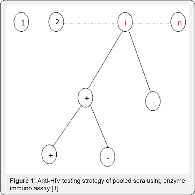
The design that is discussed here is of pooled sera as suggested by Dorfman [2]. However, the design differ from the classical pool testing in that pools that test positive are given a second test (duplicate test) as suggested by Monzon et al. [1] in their experiment as shown in Figure 1. In the pooled sera testing design, a population under investigation is of size f say pooled into n pools each of equal sizes k. The n constructed pools are then subjected to testing. Pools that test negative are dropped from further investigation. Pools that test positive are given a second screen test (duplicate test), and pools that test positive on duplicate test, constituent components are subjected to screening as shown diagrammatically in Figure 1. For purpose of estimating HIV/AIDS prevalence in a population pooled into n pools, we need not subject pools that test positive on the duplicate test to individual testing in order not to reveal the identity of the subject [7]. One would wish to subject pools that test positive initially to Western Blot (WB) or a Gold Standard test [22] but due to high cost associated with it, it is too expensive for most developing countries to mount surveys where the Gold Standard Tests are employed. Hence, more savings can be attained by just using the duplicate tests as re-ported by Monzon et al. [1] and in fact the duplicate test will minimize the error of misclassification [4].
The Moment Estimators of Prevalence
Having introduced the model to be used in estimating HIV/ AIDS-prevalence, we are now in a position to develop moment estimators. First, we establish the probability of importance in our discussion. These probabilities will be the cornerstone of our analyses. The derivation of the probability of declaring a pool as positive is

Where η is the sensitivity of the test, and ϕ is the specificity of the test by sensitivity we mean, the probability of correctly classifying a positive pool or individuals whereas specificity means, the probability of correctly classifying a negative pool or individual. These two parameters will be assumed to remain constant in the entire study, and if they are not known they can be estimated from the experiment. For example, let X1 pools be known to be defective while X2 pools are known to be non-defective. (X1 + X2 = n): The pools X1 and X2 are subjected to testing as if their status were unknown but with the sole purpose of estimating η and ϕ . Suppose X*1 pools out of X1 tests positive while X*2 pools out of X2 tests negative when the experiment is carried out, then the estimators of η and ϕ are obtained as η = X*1 /X1 and ϕ = X*2 / X2 respectively. Derivation of (1) is accomplished by the law of total probability. Notice that (1) is a composite probability, which is a function of sensitivity, specificity, pool size and the prevalence of the disease p. We also know that p ϵ [0,1] and for given and greater than 0.5 as it is the case in practice (sensitivity and specificity are always high). So,

Hence π1(p) is a bounded continuous function of p. Now the probability that a pool tests positive on the test instance and negative on re-test is

Clearly, (3) is also a function of p. Hence it can be used to estimate the prevalence as it will be shown later. As in the discussion of (2), we also have

Finally, the computation of the probability of declaring a pool as negative, denoted by π3 (p), is given as

It then follows that π3(p) is a bounded function of p

In this case, the model of interest is a multinomial. The multinomial model can be put into the exponential form and the moments easily derived. This is because multinomial distribution belongs to the exponential family (Lehman & Casella, 1995: pp. 25). The likelihood function is given by

where x1 are pools classified positive, and x2 are pools declared negative by the duplicate test,  Model (8) is of interest because our estimate of prevalence p will be based on it. We obtain the moment estimate of p from (8). As noted earlier, (8) belongs to exponential family. Thus, we have

Equation (9) implies that  respectively. We are now in a position to provide ways of estimating the prevalence p. There are three such ways. The first moment-estimator of p is based on (1) and is given by

The moment estimator of p provided by (10) is not valid for η = l -ϕ or η + ϕ = 1; a result also observed by Brookmeyer [6] that η + ϕ> 1. In such a situation, Equation (10) is valid. The second moment-estimator of p is derived from (3) is given by

Equation (11) is not valid for ϕ(1-ϕ) = η(1-η), hence it will only hold in situations where ϕ(1 -η) ≠η(1 -η) Notice that p is a poor estimator of p and the assertion is evident in Figure 2. In most practical HIV/AIDS testing situations, η2(p) is roughly zero, thus making the estimator a function of sensitivity and specificity as it can be seen in (Figures 2 & 3).
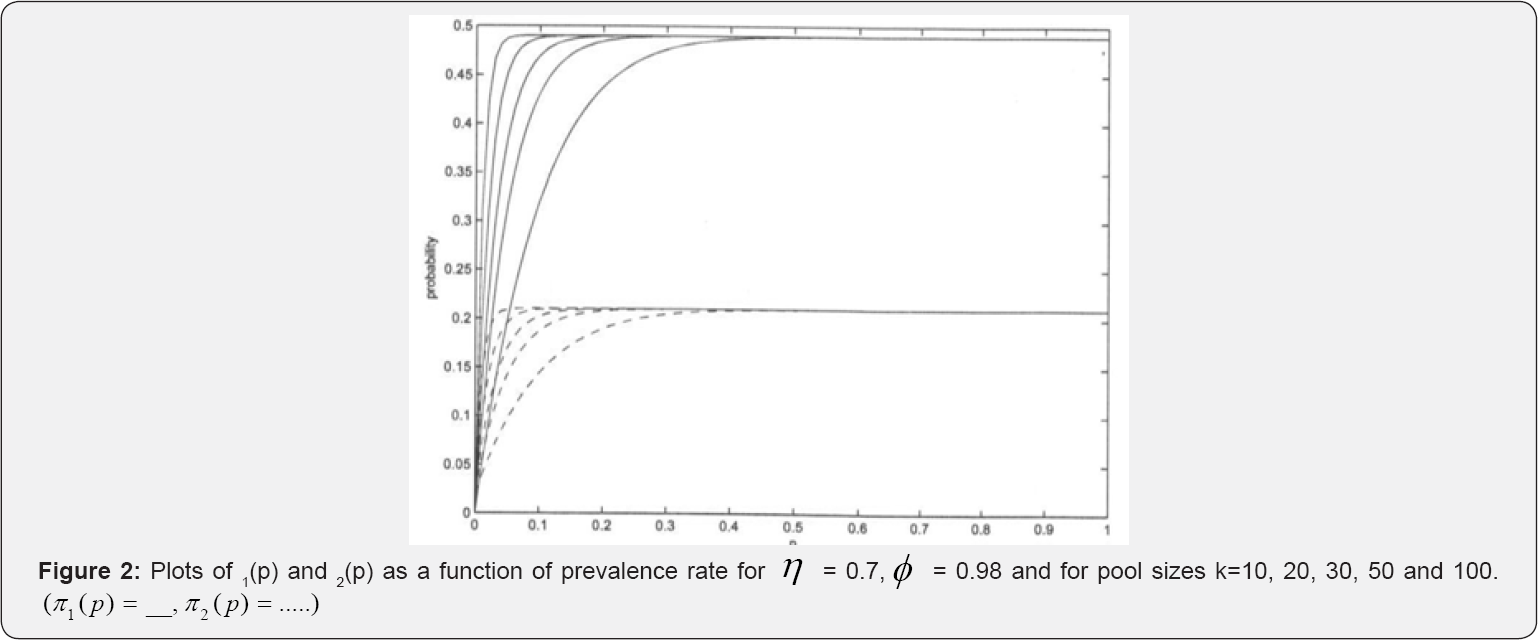
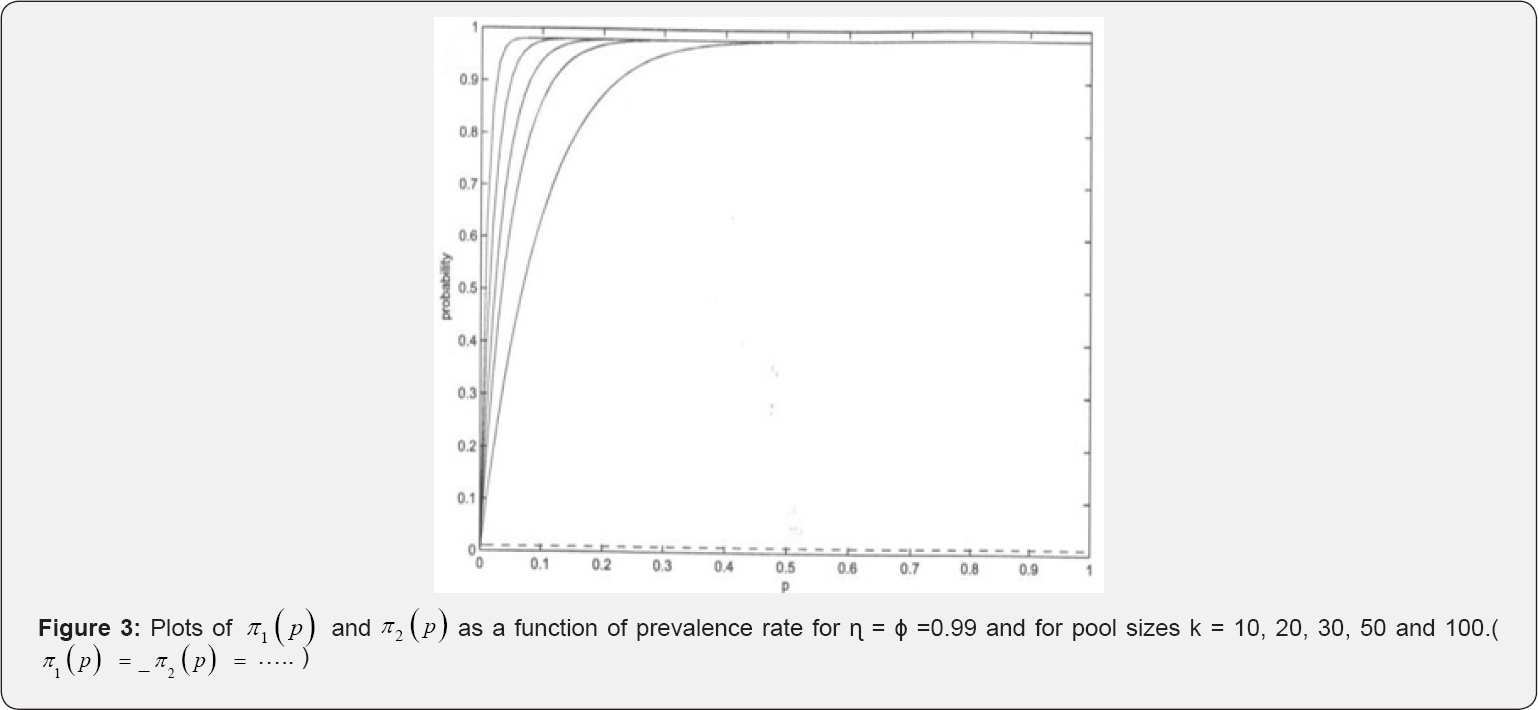
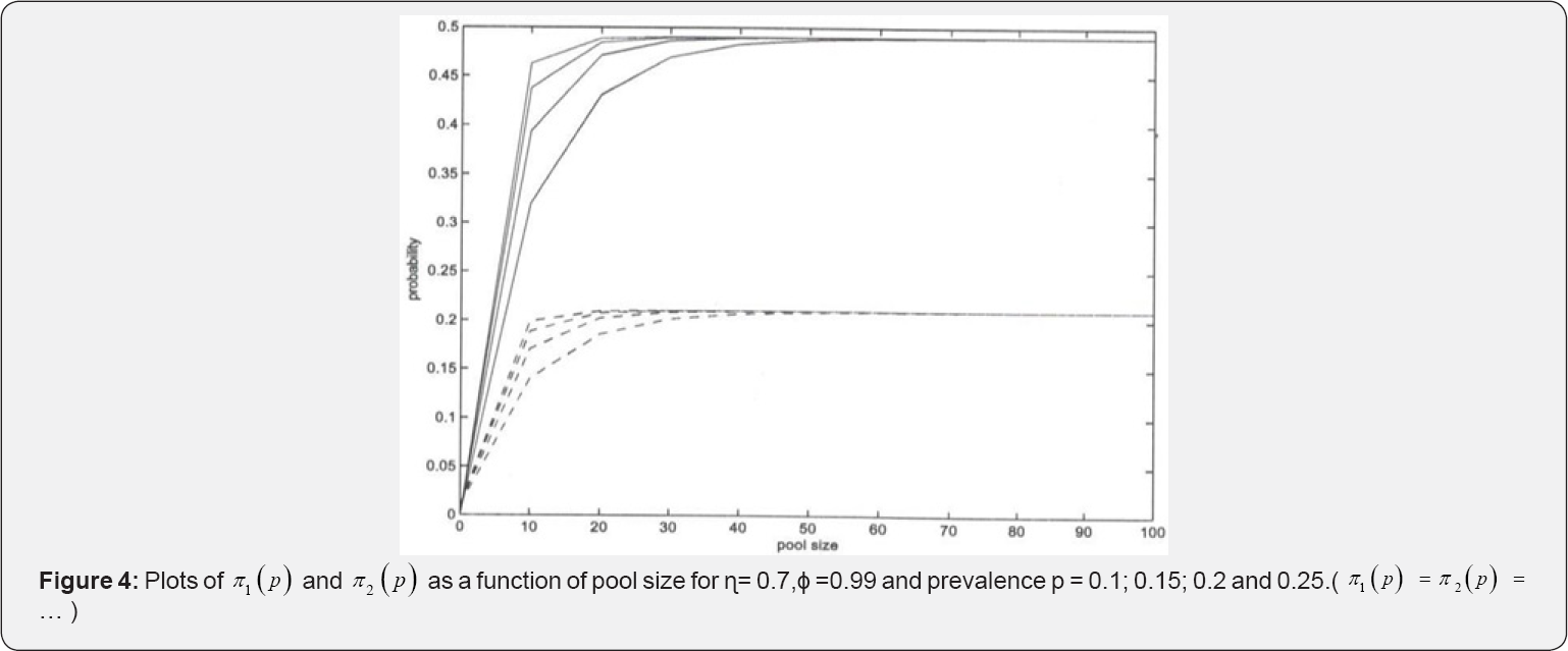
Figures 2 & 3 provides the plots of π1(p), and π2( p) versus the prevalence rate p for some selected pool sizes, sensitivity ( η ) and specificity (ϕ). From the figures we observe that π1(p), and π2(p) increases with increase in p for p ≤ 0.5 . For η = 0.7 and ϕ = 0.99, changes in π1(p), and π2(p) remain constant for p > 0.5 and p >0.4 respectively for all used group sizes. Also, we observe that π1(p), remains invariant at about π1(p) ≈0.5 while π2(p) remains invariant at about π1(p) ≈ 0.2 as shown in Figure 3. Notice that π2(p) vanishes with increase in η→1 whereas π1(p) → 1 for all investigated pool sizes. This illustrates that π2( p) is a poor estimator of p when sensitivity and specificity are high as illustrated in (Figure 3 & 4).
Plots of π1(p) and π2 (p) versus pool size (k) for some selected η, ϕ, and prevalence rate p are provided in Figure 4 above. For pool size of more than 50 variation in both π1(p) and π2(p) remains constant for η =0.7 and ϕ = 0.99. This suggests the use of small pool sizes as is the case in practice. A third moment estimator of p is

With ϕ + nη> 1. As in the case of  is the worst estimator of the prevalence. This can be checked by plotting π3( p) versus p. It is insensitive to variation in p, making it the worst estimator Therefore, this rules out two estimators namely
  as possible candidates for estimating the HIV/AIDS prevalence. Only one candidate
  is the ultimate choice for moment estimator of the prevalence and its variance is

The confidence interval (CI) for the estimator of p utilizing as the possible candidate estimator is

While the pool sizes that can minimize the variance can be computed from

Solving for k can be easily achieved by in build MATLAB functions as shown in Example 1. Now, writing the likelihood model (8) into the exponential form as
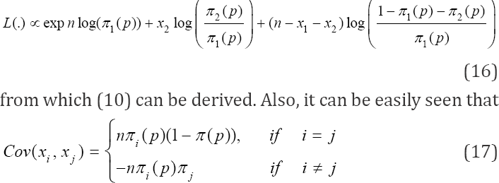
Note that we assumed tests to be independent but we have obtained estimators i.e. the moments-estimators of p that are dependent. That is to say, our estimators (10), (11) and (12) are correlated under some defined conditions. The variance covariance matrix of the moments estimators of p can be obtained by delta method [23] and it is given by
where 1 -ϕ = η or η + ϕ > 1. Also, note that if 1 -ϕ>η, we shall have negative correlation otherwise if (1 - ϕ)< η as is the case in practice. We shall have positive correlation between the probabilities πi(p) and πj (p)i ≠ j. For the computation of the bounds on the bias, we apply Taylor’s series expansion of  and
and  respectively The inequalities are obtained as

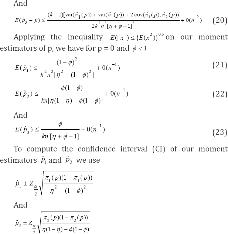
respectively. The computation of Cl can be easily implemented in statistical software as the estimates and  can be easily obtained by statistical software.
Maximum Likelihood Estimator and Asymptotic Varianc
Several moment estimators of prevalence have been presented in the preceding section. In this section, the objective is to compute a maximum likelihood estimator (MLE) of p. The MLE of ρ is traditionally obtained by maximizing/minimizing log L (.) as provided in (8). If it exists, it is unique. Our MLE of interest is computed from
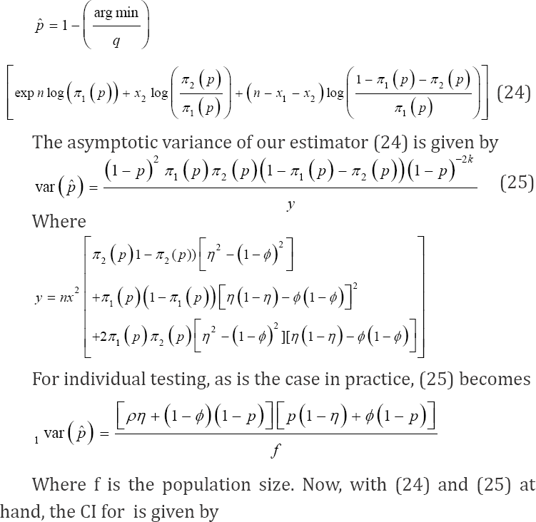
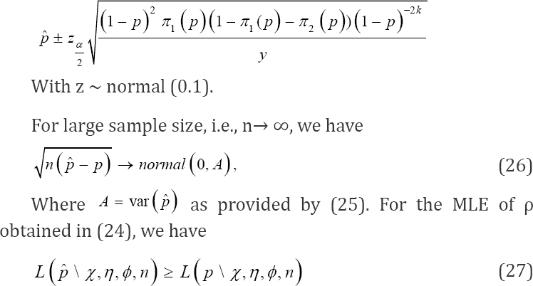
For large samples, under the assumption that the distribution tends to normality as given in (26), the estimator is the most efficient for p. Similarly, it can be easily seen that it is a sufficient estimator of p. The bias in an estimation problem is a measure of how much error we have on average. In our estimation, when we use the computed in (24) to estimate the prevalence p, the bias is given by

Notice that the computation of E ( ) from (24) is not that easy. If our estimator was unbiased, then the expected value of the estimator would be E (
 ) = p; implying that bias
  = 0: On the other hand, the mean squared error (MSE) of a given estimator is defined by

Computation of the bias and MSE in this problem can be accomplished by Monte Carlo simulations
Example 1: In this example we provide a brief history of HIV and AIDS in Kenya. Between 1983 and 1985, 26 cases ofAIDS were reported in Kenya. Sex workers were the first group affected. A study from 1985 reported an HIV prevalence of 59% amongst a group of sex workers in the capital city Nairobi. Towards the end of 1986 there was an average of four new AIDS reported to the World Health Organization each month. This, totaled 286 cases by the beginning of 1987, 38 of which had been fatal. One of the Kenya Government’s first responses was to publish informative articles in the press and launch a poster campaign urging people to use condoms and avoid indiscriminate sex. A year later in 1988, the minister of Health announced a year-long health and education programmers, funded by development partners to the tune of sterling pounds 2 million. By 1988 HIV appeared to be spreading rapidly among the population. An estimated 1.2% of adults in the capital city of Nairobi were infected with the virus, and HIV prevalence among pregnant women in the city had increased from 6.5% to staggering 13% between 1989 and 1990. By 2000 an estimated 100,000 people had already died from AIDS. And around 100 in 1000 (1 in 100) people were infected with HIV and AIDS. There have been deterring efforts in the fight of HIV and AIDS in the country and in 1999 it was declared a national disaster and the formation of National AIDS control council that was formed with the sole purpose of mobilizing resources in combating HIV/AIDS [24]. To estimate the prevalence of HIV/ AIDS in the Kenyan population using the proposed testing scheme, we assume that the test kits in use have sensitivity and specificity of 95%. The population is pooled into 100 pools each of size 10 via simple random sampling mechanism. From the computed results, we have the corresponding estimators of the HIV/AIDS prevalence as = 0.0869 and = 0.0973. Implying that. Note that the true prevalence rate is 0.1. Hence is a better estimator than, the moment estimator. In this example, we have applied our model in estimating the HIV/AIDS prevalence rate and obtained results within the CI of the true value.
Multistage Estimation Model
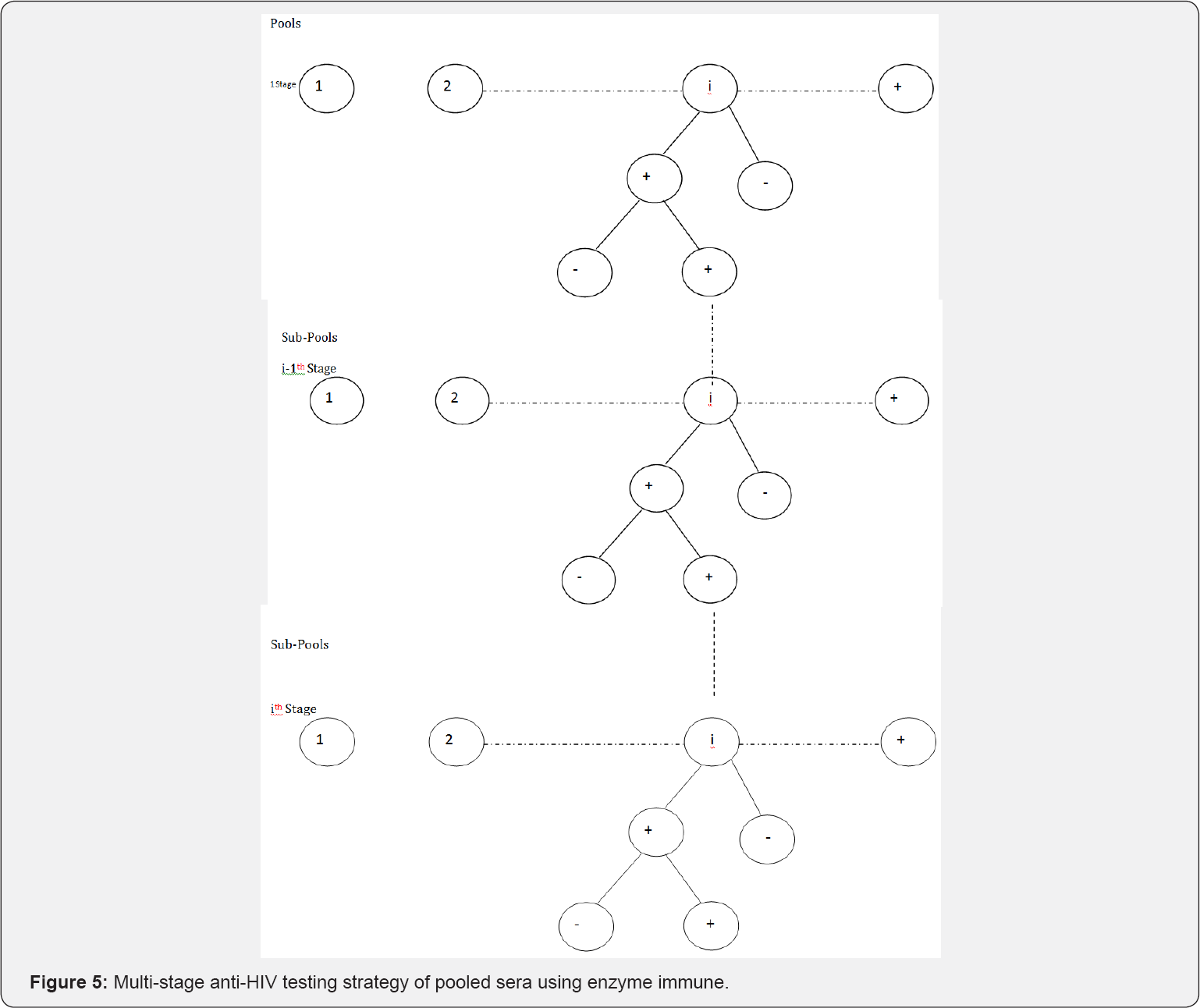
In this section, a discussion of a modified Monzon et al. [1] design as shown in Figure 1 is given. The proposed design is a generalization of the model proposed by Monzon et al. [1] this testing strategy is presented in Figure 5 diagrammatically. In the proposed design, we pool the population into n pools and each pool is subjected to testing. If a pool tests negative (-), we drop it from further investigation. If it tests positive (+) on the initial test, it is subjected to a duplicate test. If it tests negative on the duplicate test, it is dropped from further investigation. Otherwise, if it tests positive on the duplicate test, it is split into two smaller pools and the procedure is repeated on the sub-pools as shown in (Figure 5). Clearly, this is a generalization of the preceding discussion. In fact, the design discussed earlier is merely a special case as will be shown. The probability that a sub-pool is declared as positive at stage i is given

Clearly, (29) is a truncated binomial model. The model will play a major role in the formation of our MLE of p at the ith stage. The probability that a sub-pool tests positive on the initial test and tests negative on the duplicate test at the ith stage is

another truncated binomial model. Finally, the probability that a sub-pool tests negative at the ith stage is given as

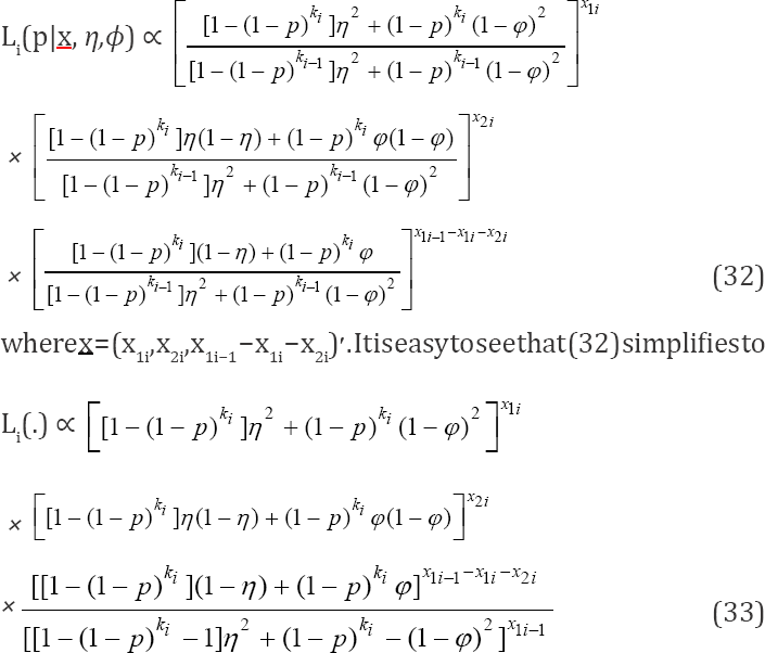
which is also a truncated binomial distribution. Therefore, the three truncatedbinomial models (29), (30) and (31) are the tools required to develop the likelihood function. It is obvious that the likelihood function will be a truncated multinomial distribution. The a likelihood function at the ith stage is given as
Thus, for the s-stage multi-stage testing scheme, the likelihood function is
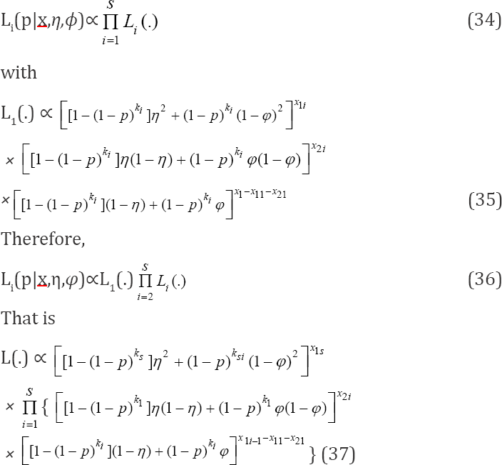
In order to obtain our estimator of interest, we must find a q = 1 - p that maximizes or minimizes (37) or its log likelihood given by

To obtain the MLE of our estimator in the proposed design, we follow similar argument as in Section 4, the MLE is accomplished by

Setting s = 1 in (37) and after intensive computation, we obtain the results as in (24). The variance obtained in (25) is the variance of the estimator when s = 1 testing scheme. Next we consider the derivation of the variance in the multistage testing strategy whose technical details are omitted. The asymptotic variance of the multistage estimator obtained in (39) is derived by applying the Crammer Rao lower bound i.e.
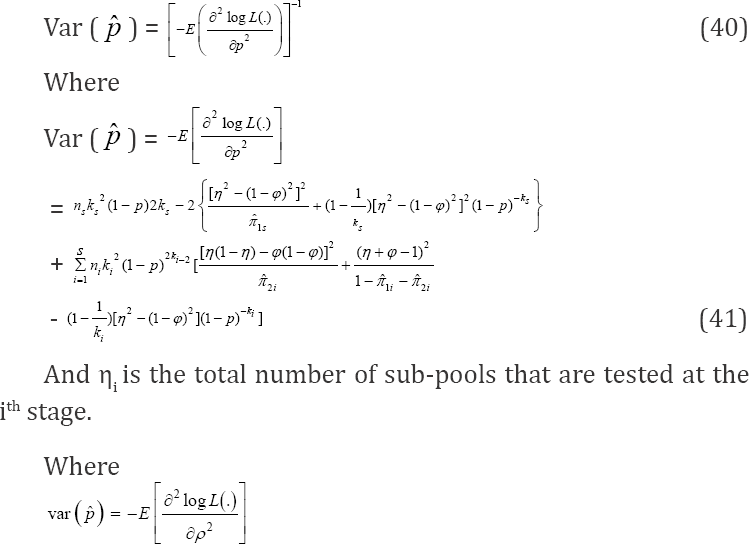
and ni is the total number of sub-pools that are tested at the ith stage. In particular, if we set s = 1 in (39) for simplicity, (25) is easily deduced. Thus, we have generalized the design proposed by Monzon et al. [1] and, at the same time, generalized both our estimator and its asymptotic variance. The large-sample property of our estimator can be studied without reference to the loss function in the multi-stage design. Therefore, approximation to or limit of performance measures as the number of pool sizes increases, i.e., n for the multi-stage model by central limit theorem (CLT) is

Where can be derived from (39) and Var (p) is obtained from (41). Also, the asymptotic relative efficiency (ARE) of the proposed multi-stage testing scheme is

Asymptotic relative efficiency (ARE) helps in assessing the efficiency of our estimator as compared to one-at-a-time testing procedure. Plots for various values of Var ( jVar (
 ) versus k are provided in (Figures 6 & 7).
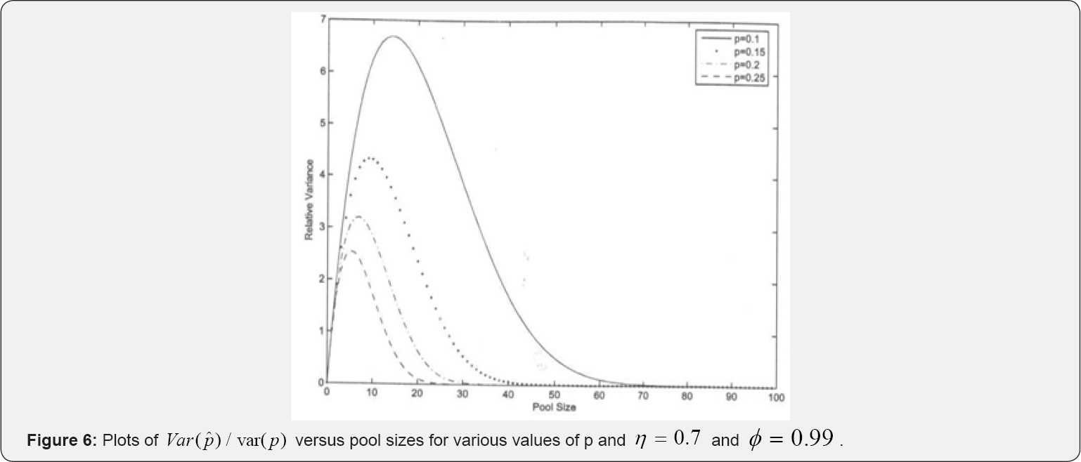
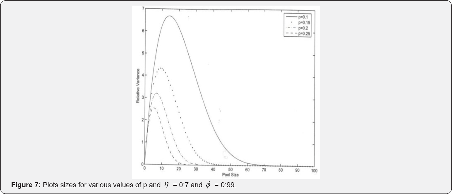
In Figure 6, we notice that the relative variances increase with increase in k up to some optimal group-size, and then drops. It also reduces with increase in p. Figure 7 shows the effect of a slight change in. In this figure, we observe that the relative variance increases with decrease in relative accuracy of the tests in use. Therefore, repeated testing model of Monzon et al. [1] should be applied in situations where the efficiency of the test kits is low for better results in practice. The multi-stage model outperforms one- at-a-time testing procedure as the AREs > 1: For instance, for only a simple case s = 1; they ARE increases with increase in pool size as it can be easily seen in Figures 6 & 7. It is therefore anticipated that as the number of stages increases the ARE will increase and MSE reduce as demonstrated by Brookmeyer [6] who investigated the problem of multi-stage estimation with perfect tests. Our study generalizes Brookmeyer [6] by introducing the error component as well as the duplicate test as it is the case in practice Monzon et

Where Var (p) is provided in (41) and for simple case where s = 1 is discussed in Section 4.
Results
We have developed estimators based on the screening design proposed by Monzon et al. [1] and extended it to the situation with sub-pooling algorithms. Although the estimator of standard screening problem holds well when the prevalence of the population is low, our approach performs better in slightly higher prevalence population. Our approach is even more robust in situations where the efficiency of the test kits are low, i.e., re-testing is preferred when the efficiency of the test kits are low as observed in the discussion. This result concurs with observations made in practice as alluded to by Sterret [25]. It is in order therefore to conclude that the procedure is viable for developing countries as retesting with the same type of kit is relatively cheap compared to the more expensive test kits like the Western Blot.
Our approach is easy to implement. At the same time it is more efficient than individual testing as observed in Figures 6 & 7. Also, the procedure is more efficient in relatively higher prevalence population than the classical pool- screening algorithms as repeated testing improves the efficiency of the testing strategy. Notice that we ruled out two possible candidates for estimating the prevalence namely  Thus we had only two candidates for consideration for estimating the prevalence, these are
  and the
  This leads to the question: which one of the two is recommended for this study? To help the discussion we compute the AREs

The variable y is provided in (23). Also, it is reported in Tu et al. [13] that the classical MLE for estimating prevalence with imperfect tests in the ordinary Dorfman [2] testing procedure is

where  is the pools classified as positive by a single test. Note that π( p) is the probability of classifying a pool as positive and is π( p) = η(1 - (1 - p)k + (1 - ϕ)(1 - p)k It can easily be seen from (12) that if π1(p) ≈ π(p), then Var
 for η = ϕ because (η2 -(1 -ϕ) 2 ))2 = (η + ϕ-1)2 for all η and ϕ(0 ≤η≤ 1,0 ≤ϕ≤ 1)- If η > ϕthen (η2 -(1 - ϕ)2 > (η + ϕ-1)2 implying that
  Hence, in such situations, the estimator
  is superior to
  of Tu et al. [13]. Similarly, if η<ϕ then (η2 - (1 -ϕ)2 < (η + ϕ-1)2, implying that
  Hence, in this case, the estimator
  is superior to
  and call for no retesting in such situations. They ARE off
  is
is

Further, comparing the asymptotic variance of  with the classical variance of
  we obtain ARE as

Simulations of the AREs for various values of p,k,η and ϕ are provided in Table 1 below. For illustration purposes, we have usedMATLAB package to compute the AREs in the table (Table 1).
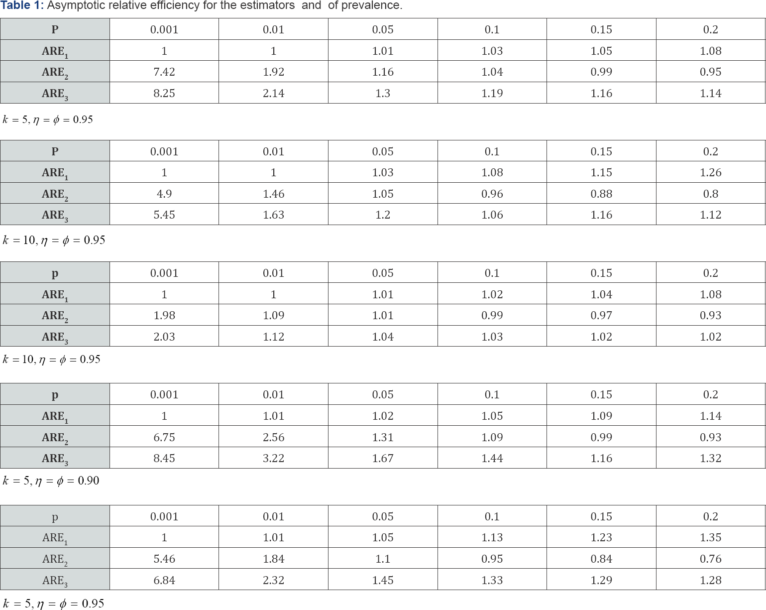
Clearly, the simulated ARE1 > 1; implying that the proposed MLE  is more efficient than the moment-estimator
  Thus,
Thus,  is more superior to
  in estimating HIV/AIDS prevalence in an African population where it is believed the prevalence is high. Also, note that ARE3 > 1 and the estimator
  is provided as the MLE of the prevalence in the past literature-i.e., Thompson [8] and Brookmeyer [6] derived
  for perfecttests and Tu et al. [13] derived
  for imperfect test. Therefore, the proposed MLE estimator is superior to the past estimators and can be recommended for screening purposes as opposed to the
  estimator common in pool-testing literature. It can be easily noticed from the tabulated results that the proposed MLE estimator becomes superior to
  when the prevalence of the population is small, calling for re-testing when the prevalence of the population is low. That is, retesting is recommended for high risk population Nyongesa [21]. Also, it is easily seen that the proposed MLE is more efficient in situations where the sensitivity and specificity are low. For ARE2 > 1; meaning that
 is more efficient than
  and this complicates the applicability of
  in estimating HIV/AIDS in low prevalence populations confounded with the fact that there is loss of sensitivity when pooling strategies are applied in screening HIV/ AIDS Kline et al. [3] and the loss in sensitivity can be recovered by retesting. The ARE2 < 1 for high prevalence rates such as 0.2 makes
  a poor estimator. For example, if the prevalence of the population is 0.15, the ARE2 is 0.88 when k = 10, η = ϕ = 0.95, thus for ARE2 < 1 makes
  a poor estimator of prevalence in high prevalence population [26].
Conclusion
This study proposed moment estimators for prevalence estimation and MLE. It has been demonstrated that the proposed ME p^1 is superior to the studied p^G in some situations whereas the MLE p^ outperform both p^1 and p^AG. More efficient estimators can be realized if multi-stage models are applied. However, multistage models are only possible if there enough samples to allow creation of sub-pools. The study only discussed halving multistage model but a generalized multi-stage model that allows creation of any number of sub-pools at any stage can be studied and results compared with the one proposed in this study
References
- Mitchel S, Monzon OT, Paladin E, Fem Julia P, Dimaandal E, et al. (1992) Relevance of antibody content and test format in HIV/AIDS testing of pooled sera. AIDS 6(1): 43-48.
- Dorfman R (1943) The detection of defective members of large population. Annals of Mathematical Statistics 14(4): 436-440.
- Kline RL, Bothus TA, Brookmeyer R, Zeyer S, Quinn TC (1989) Evaluation of human Immunodeficiency virus sero prevalence in population surveys using pooled sera. J Clin Microbiol 27(7): 14491452.
- Nyongesa LK (2004) Multistage group testing procedure (Group screening) Communication in Statistics-Simulation and computation. 33(3): 621-637.
- Johnson Nl, Kotz S, Wu X (1991) Inspection errors for attributes in quality control. London; Chapman and Hall, UK.
- Brookmeyer R (1999) Analysis of multistage pooling studies of Biological specimens for Estimating Disease Incidence and prevalence. Biometric 55(2): 608-612.
- Gastwirth JL, Hammick PA (1989) Estimation of the prevalence of a rare disease preserving the anonymity of the subject by Group-testing; Application to estimating the prevalence of AIDS antibodies in blood donors. Journal of statistical planning and inference 22(1): 15-27.
- Thompson KH (1962) Estimation of the population of vectors in a natural population of insects. Biometrics 18(40029): 568-578.
- Sobel M, Elasho RM (1975) Group-testing with a new goal estimation. Biometrika 62(1): 181-193.
- Behets F, Bertezzi S, Kasali M, Kashamuka M, Atikala L, et al. (1990) Successful use of pooled sera to determine HIV/AIDS-1 seroprevalence in Zaire with development of cost-effective models. AIDS 4(8): 737741.
- Gastwirth JL, Johnson WO (1994) Screening with cost-effective quality control: Potential applications to HIV/AIDS and drug testing. Journal of the American Statistical Association 89(427): 972-981.
- Hammick PA, Gastwirth JL (1994) Extending the applicability of estimation of prevalence of sensitive characteristics by group testing to moderate prevalence populations. International Statistical Review 62: 319-331.
- Tu MX, Litrak E, Pagano M (1995) On the in formativeness and accuracy of pooled testing in estimating prevalence of a rare disease: Application to HIV/AIDS screening. Biometrika 82(2): 287-297.
- Xie M, Tatsuoka K, Sacks J, Young S (2001) Group testing with Blockers and synergism. Journal of American Statistical Association 96(453): 92-102.
- Tebbs MJ, Swallow HW (2003) Estimating ordered binomial proportions with the use of group testing. Biometrika 90(2): 471-477.
- Swallow WH (1985) Group testing for estimating infection rates and probability of disease transmission. Phytopathology.
- Hung M, Swallow (2000) Use of binomial group testing in tests of hypothesis for classification or quantitative covariates. Biometrics 56(1): 319-331.
- Ding J, Xiong W (2015) Robust group testing for multiple traits with miscalculation. Journal of Applied Statistics.
- Okoth AW, Nyongesa LK, Kwatch BO (2017) Multi-stage adaptive pool-testing model with Test errors; Improved efficiently. Journal of Mathematics 13(1): 43-55.
- Matiri G, Nyongesa K, Ali I (2017) Sequentially Selecting Between Two Experiment for Optimal Estimation of a Trait with Misclassification. American Journal of Theoretical and Applied Statistics 6(2): 79-89.
- Nyongesa LK (2004b) Testing for the Presence of Disease by Pooling Samples. Australian and New Zealand Journal of Statistics 46(3): 383390.
- Johnson WO, Pearson LM (1999) Dual Screening. Biometrics 55(3): 867-873.
- Billingsley P (1995) Probability and measure (3rd edn) John Wiley and Sons Inc, New Jersey, United States.
- (2005) National AIDS Control Council Kenya National HIV/AIDS Strategic Plan (KNASP).
- Monzon OT, Palalin FJ, Dimaal E, Balis AM, Samson C, et al. (1957) On the detection of defective members of large population. Annals of Mathematical Statistics 28(4): 1033-1036.
- Lehmann El, Casella G (1998) Theory of point Estimation (2nd edn) Springer Verlag, New-York Inc, USA.


