petrochemical science journal | Juniper Publishers

Facing Challenges on Demand Forecasting: Dealing With Short Data in the Petrochemical Industry

Pinheiro MAP¹*, Delmonico DVG², dos Santos HH², Fadel RF¹ and Medola SHC¹

¹Department of Production Engineering, Brazil

²Department of Production Engineering, Sao Paulo State University, Brazil

Submission: April 16, 2018; Published: April 30, 2018

*Corresponding author: Pinheiro MAP, Faculty of Agudos, Av Marginal Vereador Delfino Tendolo, Agudos/SP-Brazil, Brazil, Email: marco.pinheiro@faag.com.br

How to cite this article: Pinheiro MAP, Delmonico DVG, dos S HH, Fadel RF, Medola SHC. Facing Challenges on Demand Forecasting: Dealing With Short Data in the Petrochemical Industry. Recent Adv Petrochem Sci 2018; 5(1): 555655. DOI: 10.19080/RAPSCI.2018.05.555655

Abstract

This article aims to verify how a fuels distributor industry operates and plans forecast demand for gasoline and diesel, which are responsible for most of the operating losses. Through a case study, the findings suggest that the company has a shortage in this process, considering that does not use mathematical models and methods or specific systems in the industry to make decisions, based only on the opinion and advice of managers. The research results has shown that the application of known techniques of forecasting can bring some advantage to the organization, understanding that only knowledge and professional experience are factors that should not be worked out in a standardized manner. Its association with mathematical models and methods can improve the company's result.

Keywords: Short data; Demand forecasting; Fuel industry; Simple moving average; Exponential smoothing demand forecasting

Introduction

Forecasting future demands is asignificantactivity for any economic sector. Market forecasting capabilities may be relevant to good business performance [1]. Although formal methods contribute to forecasting demand, many firms still rely on less formal forecasting methods [2]. In this sense, demand forecasting is the function that is the source of demand signal distortions [3]. The forecast function is alsoessential both for inventory management in industries [4] and for efficiency in [5], and for the parts marketing market [6].

Despite an old theme that develops at a certain speed, demand forecasting uses time-series analysis techniques. More recently, well-accepted academic production on demand forecasting has used methods such as neural networks [7-9]. However, with the correct updates, other more straightforward methods are still being studied, such as the moving average [10] and exponential smoothing [11], considered a classical method developed from the moving average [12].

The literature on demand forecasting, in general, presents some characteristics that do not help everyday practical situations of small companies. The studies in the area of demand forecasting indicate a strong orientation towards large markets, such as electric sector [13,14] and water sector [5]. Moreover, in a preliminary perspective, studies on themes such as moving average and exponential smoothing suggeststudies oriented towards the development of the method [15]. The literature is also indicating a predominance of the use of large sectors, such as energy [16] and capital markets [11] as sources of empirical data and cases analyzed.

The literature has already observed the study of forecast fuel demand [17], focusing on the domestic market. According to the authors, the prediction of fuel demand gets attention from the oil crisis in the 1970s and is the focus of environmental concerns and energy planning. Thus, adequate demand management by distributors has the potential to minimize general problems in inventory management. Also, it also assists in the financial planning of distributors.

In this vein, the objective of this article is to analyze the application of simple methods of forecasting demand for analysis of short historical series in a Brazilian fuel distributor. For this, a historical data survey was carried out with elements of case studies in a company in the countryside of the State of Sao Paulo. From the results, the two classic demand forecast models, the moving average, and the exponential smoothing were compared. Also, methods will be discussed in contrast to the intuitive prediction performed by the entrepreneur. Among the main contributions of the work.

Conceptual Background

The recent literature presents demand forecasting as the best estimation of future demand for companies, given a set of assumptions [18]. From what Song & colleagues [19] point to the electric sector, it can be said that the calculation of the demand forecast uses characteristics of the object of study, as well as data of time series, correlations between the demand of that sector and economic factors.

The recent studies suggest the concentration of the demand forecasting studies on broader areas, such as the electric sector [20,21]. The focusing on the electric sector includes studies on short-term valuation from aggregate demand [13], and medium and long-term using big data in an intelligent city [22]. Thus, the literature also focuses in the consumption [23], integration with industrial capacity [19], and household consumption forecast from a conditional density estimation [14], also articles involving various estimation methods [24].

Time-series analysis for demand forecasting uses several methods. With updates for types of analysis and various kind of variables involved, the literature still uses the classic models such as moving average and exponential smoothing. Upgrades of the moving average model, include the autoregressive moving average (ARMA), the periodic autoregressive moving average (PARMA), the adaptive ARMA model [20], among others.

Recent articles include the moving average as a method of analysis, such as Fingleton et al. [25] that used the spatial moving average associated with other ways in European Union unemployment data. Tang et al. [26] contributed to the development of the exponentially weighted adaptive moving average proposing a new control table. Strobel & Auer [27] demonstrated how the variable moving average (VMA) lost the explanatory capacity to predict changes in market prices in the US stock market. Dias and Kapetanios [10] used the autoregressive vector moving average (VARMA) in the study of macroeconomic data using large datasets.

Exponential smoothing, in turn, is a simple technique used to smooth and predict a time series without the need to fit a parametric model [28]. Also, exponential smoothing is assumed a simple and robust method for prediction [29] and in the early years of the past decade its use was expanding and becoming generalized [30].

The recent literature on demand forecasting using exponential smoothing has studies comparing several models, not only for exponential smoothing but also for moving average models [16], pointing out some limitations of the classical model. Other articles develop the method proposing a Myriad Sequential Smoothing model for the signal processing approach [31] . Also, exponential smoothing was used to develop an online programming method [15] and emission of solar irradiation [32] .

Materials and Methods

In this article, a methodology of mixed research was applied using quantitative and qualitative elements, allowing an improvement of the information [33]. For this, in the qualitative approach an exploratory research was conducted to providemore familiarity with the problem, allowing and facilitating the construction of hypotheses [34], followed by a case study, which according to Yin [35] is a research method that has a broad scope and the adequate approach to the collection and analysis of specific data.

In the quantitative approach, a simulation for the demand forecast, an object of the case study was carried out. Numerical methods analyze the simulation models and not by analytical methods. Analytical methods apply mathematical deductive reasoning to «solve» the model. In the case of Simulation models, which employ numerical methods, the models are «rotated», rather than solved [36]. The data was gathered through interviews conducted with the Director and the Operational Manager at meetings. Other data sources include documents provided by the managersand observation of the processes. The company in question is a petrochemical distributor of fuels and oil products, which operates in distribution in the state of Sao Paulo, acting more precisely in the interior of the state, southwest region. It has about 600 active clients and 2,500 registered clients, with 100% of its capital being national.

Through structured interviews and data collection and management system information, it was verified that in the first four months of 2016 the company had issues on the supply side. ThePetrobras (Petroleo Brasileiro S / A), the main (and practically sole) supplier of Diesel and Gasoline in Brazil, had difficulties in meeting the requests of the company, causing significant operational failures, in which the organization had its orders reduced in volume, causing disruptions to the attendance of its sales [37].

It was also identified that the forecast of demand in the company is made in a purely intuitive way, not using tools and methods proven effective. In this study, the focus will be only on the sales of common and additive S-500 Diesel, common S-10 diesel and additive and the common and additive Gasoline C.

Discussion

After analyzing the data and crossing it with the information provided in the interview with the operational manager, the most significant problem identified was that the company has its forecast of the demand made mainly by the knowledge and expectations of its managers, not using any system or mathematical method. It was then sought to present subsidies and demonstrate that organization should review its methodology, aiming at improvement and improvement of its forecasts.

In the first step, it was necessary to choose the model of the forecast of demand more appropriate to the organization, which model should encompass the given data amount and variables to provide the most reliable information and with the lowest possible error rate.Thus, it was needed to demonstrate the advantages of obtaining a forecast closer to reality, which can facilitate company planning in both financial and commercial aspects.The next step in the choice of the model is merely the monitoring and control of information.Because if the chosen model starts to show very high variations, with significant errors, it is evident that a reassessment will be necessary, even if it is possible to select another one model, or by reanalysis of data and information that may be causing such distortions.

Assuming that each group has its way of operating and acting, no unique forecasting model works for every market or company. In this sense, there are more coherent models with more suitable application to specific segments.What is needed is the understandingof the importance of proper planning, with integration between areas and particular attention to demand forecasting, as this information can mean the maintenance and solidity of a company, allowing the company became more competitive and prepared for the market and future actions that may occur without prior notice or preparation.

Ordinary small business organizations barely use demand- forecasting models; probably there is software for this purpose, the simple models for demand forecasting are suitable.In this sense, the chosen model is one of the more comfortable application, the Simple Moving Average (SMA). SMA is a model of clear understanding and use, and that allows practitioners to achieve results satisfactorily. The same is also recommended and used as an indicator in the graphical analysis of the stock exchange (BOVESPA), for example, helping in the study of currency fluctuations, futures contracts, stocks and so on. The basic formula for Simple Moving Average is:

For which:

V= Values of each Period

n= Total number of periods considered

With each new period, the same is added to the sum of the numerator and the first period used is neglected. For the use of the simple moving average, one must define the number of periods that will be established as parameters for the forecasts. The higher the number of periods, the tendency is that the forecast has greater assertiveness, in this way, it was established that the calculation would be done following three different sample sizes. As the analysis will be monthly, the calculations were performed based on 3, 4 and 5 months. The table below shows the organization's sales data for the period from September 15 to September 16 (Table 1 & Figure 1).

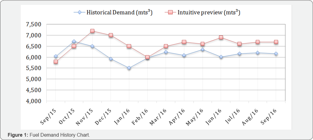
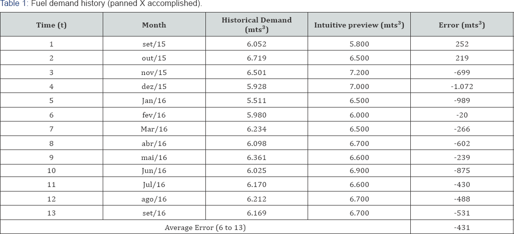
It can be seen that the average error of the period considered for the Demand Forecast calculations, from 6 to 13, was 431m³ less. The relation of the data obtained through the figure of lines in 2 dimensions is visually verified, showing the great variation between the forecast estimated by the company in comparison to the volume sold. When entering the same data in a demand forecast model using the Simple Moving Average, we will obtain: (Table 2)

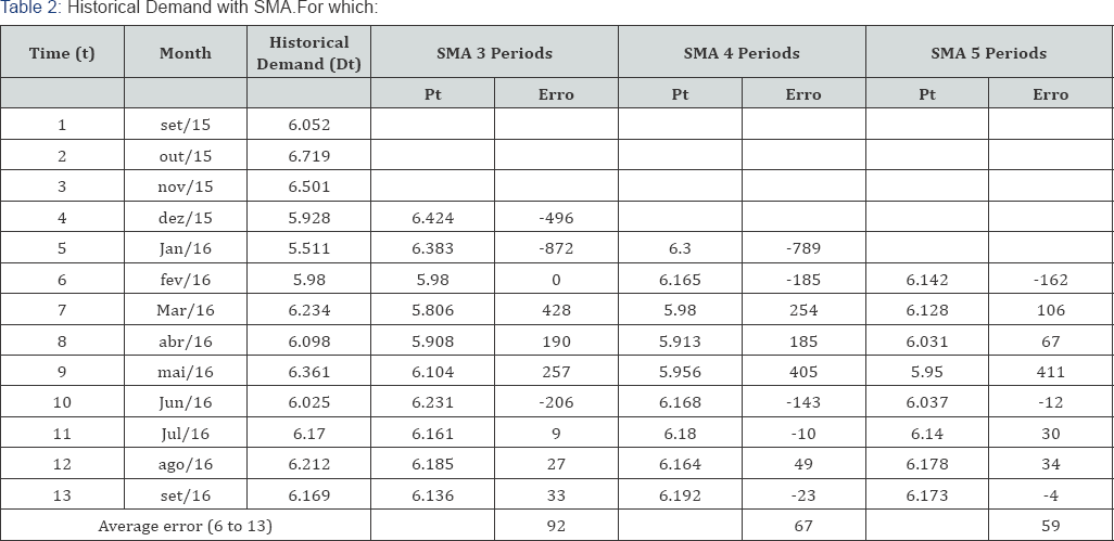
Dt = Historical demand for a given period;

Pt = Forecast for a given period

Error = Difference between the Effective Value of the Demand and the Forecast obtained. The line graph (Figure 2) shows the use of the SMA method and its results:

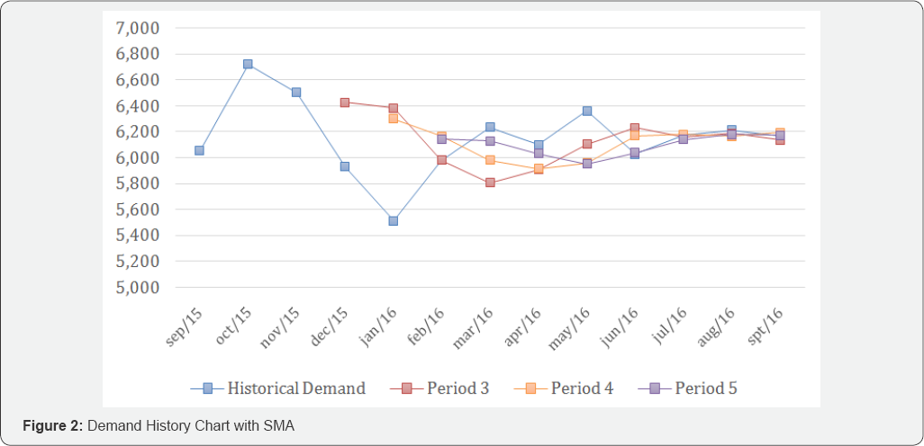
The model based on the Simple Moving Average is useful as it shows the analysis of the tables and graphs. The worst result presented in the MMS was based on three periods, with an average error of 92m³, compared to the result obtained in the real situation of the organization, the MMS was four times lower than the real error. Thus, it is evident the need for the organization to implement a forecast model of demand.

The simple exponential smoothing method may be another alternative for forecasting demand. Its simplicity of application, ease of adjustment and good precision are justifications for its full use [34]. Its form consists in assigning different weights to each observed value in a time series, assigning higher weights to more recent values. Its mathematical formulation is presented as follows:

The value of a is arbitrary, anditerativity is a way of defining which is the best value to use. The value of a that minimizes the mean of the errors can be used in the final model. In this case, values of 0.3, 0.5 and 0.8 were arbitrated. Another issue with this method is the initial estimate of the value of the last forecast. This calculation can do through a historical average of the available dataora subjective assignment can be done [34]. In the survey, the average of the available data was estimated and used as the factor of the last forecast (Table 3).

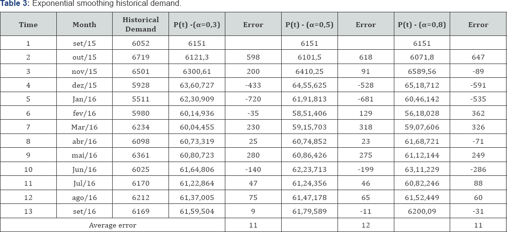
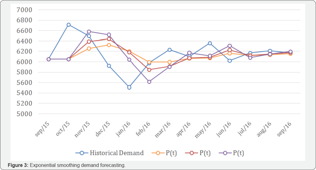
Thus, the values of the exponential smoothing were calculated for the different attributions of a: Observing the results of the table, we can notice that the different values of a did not bring significant discrepancies in the mean errors of the forecast calculations, that is, any amount used may be appropriate to the model. Figure 3 assists in understanding the pattern established by smoothing.

It is noted that the results of simple exponential smoothing presented better adjustments than the simple moving average method, but the application of any of the methods could bring much more coherent and effective information to the distributor than simply using intuitivemethod, without mathematical bases.

Conclusion

The knowledge and the professional experience within a given field of activity cannot be disregarded. Nor can the importance and influence of managers in decision-making about demand forecasting be reduced. However, this article has demonstrated the importance of implementing systematic methods and mathematical models, even if simple, to make decisions related to demand forecasting. If the company under study had made use of a simple model, its operations could have been less impacted by prediction errors.

The results represent only a part of the variables necessary to calculate the real values of gain obtained, because with the application of the SMA the average would be negative and may cause supply disruptions to customers, generating losses difficult to measure, or even the company having to acquire the product of its competitors at much higher prices, only to avoid disruptions. However, with the use of a very simple method, it was evident the achievement of the objective of this work that was to highlight the possibility of a great operational and financial gain for the company.

To illustrate the possibility of monetary gains, considering only the period of the last 8 months operated by the company in comparison to the results obtained through the use of SMA (5 periods), the average monthly error fell from 431m3 to -59m³. Only considering the average operating cost of product maintenance (storage in tanks) that in this period was approximately US$3,06 per m³ (1USD = R$3,27), the company would have an approximate cost reduction of US$ 1.318.04 per month. As the data includes 2 products of different prices it is not possible to specify the exact amount of capital employed to purchase them, but could have varied from US$ 296.559,63 to R $ 415.183,48 since in the period the value of Diesel was approximately US$0,69 and Gasoline US$ 0,96 per liter.

A professional who is well-informed, attentive and with an excellent perception of market trends, can and should influence decision making, since such a professional can anticipate events without a history of occurrence, can perceive a change of market trend, that is, there are innumerable situations that may occur and that a system would not be able to predict, but preferably, it should do so with the support of a mathematical forecasting system / model.

Through the literary review it was realized that the forecast of demand is relevant for the better administration of materials, because with it occurs decrease of errors, consequently increasing the productivity and business gains. One of the limitations of this research is the use of only two models for the simulation of demand forecasting, which may distort the results somewhat. Suggestions for future studies consider the application of more robust methods such as Weighted Moving Average, since the method tendsto be more assertive because it treats and considersa greater number of factors, such as seasonality and other variables.

References

- Moon M, Mentzer J, Smith C (2003) Conducting a sales forecasting audit. International Journal of Forecasting 19(1): 5-25.
- Baecke P, Baets DS, Vanderheyden K (2017) Investigating the added value of integrating human judgement into statistical demand forecasting systems. International Journal of Production Economics 191: 85-96.
- Carbonneau R, Laframboise K, Vahidov R (2008) Application of machine learning techniques for supply chain demand forecasting. European Journal of Operational Research 184(3): 1140-1154.
- Bergman JJ, Noble JS, McGarvey RG, Bradley RL (2017) A Bayesian approach to demand forecasting for new equipment programs. Robotics and Computer-Integrated Manufacturing 47: 17-21.
- Gagliardi F, Alvisi S, Kapelan Z, Franchini M (2017) A probabilistic short-term water demand forecasting model based on the markov chain. Water 9(7): 507.
- Bacchetti A, Saccani N (2012) Spare parts classification and demand forecasting for stock control: Investigating the gap between research and practice. Omega 40(6): 722-737.
- Jiang S, Chin KS, Wang L, Qu G, Tsui KL, et al. (2017) Modified genetic algorithm-based feature selection combined with pre-trained deep neural network for demand forecasting in outpatient department. Expert Systems with Applications 82: 216-230.
- An N, Zhao W, Wang J, Shang D, Zhao E, et al. (2013) Using multi-output feed forward neural network with empirical mode decomposition based signal filtering for electricity demand forecasting. Energy 49(1): 279-288.
- Al-Saba T, El-Amin I (1999) Artificial neural networks as applied to long-term demand forecasting. Artificial Intelligence in Engineering, 13(2): 189-197.
- Dias GF, Kapetanios G (2018) Estimation and forecasting in vector autoregressive moving average models for rich datasets. Journal of Econometrics 202(1): 75-91.
- Snyder RD, Koehler A, Ord K (2015) Forecasting for inventory control with exponential smoothing forecasting for inventory control with exponential smoothing. International Journal of Forecasting 18(1): 5-18.
- Guo F, Diao J, Zhao Q, Wang D, Sun Q, et al. (2017) A double-level combination approach for demand forecasting of repairable airplane spare parts based on turnover data. Computers and Industrial Engineering 110: 92-108.
- Al-Musaylh MS, Deo RC, Adamowski JF, Li Y (2018) Short-term electricity demand forecasting with MARS, SVR and ARIMA models using aggregated demand data in Queensland, Australia. Advanced Engineering Informatics, 35: 1-16.
- Amara F, Agbossou K, Dube Y, Kelouwani S, Cardenas A, et al. (2017) Household electricity demand forecasting using adaptive conditional density estimation. Energy and Buildings, 156: 271-280.
- Heger J, Grundstein S, Freitag M (2017) Online-scheduling using past and real-time data. An assessment by discrete event simulation using exponential smoothing. CIRP Journal of Manufacturing Science and Technology 19: 158-163.
- Oliveira DEM, Oliveira CFL (2018) Forecasting mid-long term electric energy consumption through bagging ARIMA and exponential smoothing methods. Energy 144: 776-788.
- Li Z, Rose JM, Hensher DA (2010) Forecasting automobile petrol demand in Australia: An evaluation of empirical models. Transportation Research Part A: Policy and Practice, 44(1): 16-38.
- Rosienkiewicz M, Chlebus E, Detyna J (2017) A hybrid spares demand forecasting method dedicated to mining industry. Applied Mathematical Modelling 49: 87-107.
- Song Z, Niu D, Dai S, Xiao X, Wang Y, et al. (2017) Incorporating the influence of China's industrial capacity elimination policies in electricity demand forecasting. Utilities Policy 47: 1-11.
- Vu DH, Muttaqi KM, Agalgaonkar AP, Bouzerdoum A (2017) Shortterm electricity demand forecasting using autoregressive based time varying model incorporating representative data adjustment. Applied Energy 205: 790-801.
- Hu YC (2017) Nonadditive grey prediction using functional-link net for energy demand forecasting. Sustainability, 9(7): 1166.
- Wei Z, Li X, Li X, Hu Q, Zhang H, et al. (2017) Medium- and long-term electric power demand forecasting based on the big data of smart city. Journal of Physics: Conference Series 887(1).
- Shao Z, Chao F, Yang SL, Zhou KLe (2017) A review of the decomposition methodology for extracting and identifying the fluctuation characteristics in electricity demand forecasting. Renewable and Sustainable Energy Reviews 75: 123-136.
- Yoshida A, Yoshikawa J, Fujimoto Y, Amano Y, Hayashi Y, et al. (2018) Stochastic Receding Horizon Control Minimizing Mean-variance with Demand Forecasting for Home EMSs. Energy and Buildings 158: 16321639.
- Fingleton B, Gallo LJ, Pirotte A (2017) A multidimensional spatial lag panel data model with spatial moving average nested random effects errors. Empirical Economics, pp. 1-34.
- Tang A, Castagliola P, Sun J, Hu XL (2017) An adaptive exponentially weighted moving average chart for the mean with variable sampling intervals. Quality and Reliability Engineering International 33(8): 2023-2034.
- Strobel M, Auer BR (2018) Does the predictive power of variable moving average rules vanish over time and can we explain such tendencies? International Review of Economics and Finance 53:168184.
- Gelper S, Fried R, Croux C (2010) Robust forecasting with exponential and holt-winters smoothing. Journal of Forecasting, 29(3): 285-300.
- Billah B, King ML, Snyder RD, Koehler AB (2006) Exponential smoothing model selection for forecasting. International Journal of Forecasting 22(2): 239-247.
- Taylor JW (2003) Exponential smoothing with a damped multiplicative trend. International Journal of Forecasting 19(4): 715-725.
- Goh BMK, Lim HS, Tan AWC (2017) Exponential myriad smoothing algorithm for robust signal processing in a -stable noise environments. Circuits, Systems, and Signal Processing, 36(11): 4468-4481.
- Dong Z, Yang D, Reindl T, Walsh WM (2013) Short-term solar irradiance forecasting using exponential smoothing state space model. Energy 55: 1104-1113.
- Creswell JW (2010) Projeto de pesquisa metodos qualitativo, quantitativo e misto. In: Projeto de pesquisa metodos qualitativo, quantitativo e misto. Artmed.
- Pellegrini FR, Fogliatto FS (2001) Passos para implantafao de sistemas de previsao de demanda-tecnicas e estudo de caso. Produfao 11(1): 43-64.
- Yin RK (2015) Estudo de Caso-: Planejamento e Metodos. In: (5th edn), Bookman editora.
- Banks J (1996) Discrete-Event System Simulation. Prentice Hall. New Jersey, USA.
- Alvisi S, Franchini M, Marinelli A (2007) A short-term, pattern-based model for water-demand forecasting. Journal of Hydroinformatics 9(1): 39-50.