


A Comparison of CMM and CMA Capabilities in Product Feature Verification Metrology
Cesar Miguel Marquez Rodriguez and Shivakumar Raman*
Department of Industrial Engineering, University of Oklahoma, Norman, OK, USA
Submission:June 16, 2023; Published:July 07, 2023
*Corresponding author:Shivakumar Raman, Department of Industrial Engineering, University of Oklahoma, Norman, OK, USA Email: raman@ou.edu
How to cite this article: Cesar Miguel Marquez R, Shivakumar R. A Comparison of CMM and CMA Capabilities in Product Feature Verification Metrology. Robot Autom Eng J. 2023; 5(4): 555667. DOI: 10.19080/RAEJ.2023.05.555667
Abstract
To control variations and guarantee that a part will function as intended in an assembly, measurement verification must be conducted with specialized metrology equipment. The Coordinate Measuring Machine (CMM) and the Articulated Arm CMM (AA-CMM) are analyzed in this comparative study, to identify their respective advantages and disadvantages when measuring flatness. The goal of this pilot study is to detect the measuring limitations of each machine and propose a methodology to identify appropriate use of each device based on its capabilities. For measuring flatness, contact and contactless measurement experiments were designed. As expected, it is observed that the CMM performs better than the CMA in flatness measurement because it has a higher resolution [1]. By looking at the measured flatness obtained during the experiment, it was determined that the CMM had a smaller minimum measurable tolerance in all permutations of the test when compared to its counterpart. Resulting in the proposal of different functional working envelopes for these machines. Establishing working envelopes permits the use of both machines for overlapping working purposes as the versatility of CMAs in Geometry verification in settings where CMMs cannot be deployed, could have a great impact as long as they operate on the corresponding working envelopes defined in this research, which were defined as follows: CMM has a minimum measurable tolerance of 0.0006in, CMA contact, has a minimum measurable tolerance of 0.0024in and CMA contactless, has a minimum measurable tolerance of 0.0045in.
Keywords: CMM; AA-CMM; CMA; Laser Point; Metrology device selection; Measurement boundary; Flatness verification
Resolution: The smallest difference in dimensions that the measuring instrument can detect or distinguish.
Introduction
Quality control has become a paramount process in most industries and successful organizations. In the manufacturing sector, “products develop certain external and internal characteristics that result, in part, from the type of production processes employed” [2]. Metrology science has defined those characteristics over the years and established methods and processes to inspect manufactured parts and guarantee that they meet specifications. Usually, “external characteristics relate to dimensions, size, surface finish, and integrity; while internal characteristics include defects like porosity, impurities, inclusions, residual stresses, among others” [2]. These deviations are normal and expected, as it is virtually impossible to reproduce a part without variation. Therefore, in manufacturing, fabricated pieces are allowed to show characteristics that fall within a defined range known as tolerance.
One of the ways we can evaluate the parts, and consequently the performance of the process and the machines used, is by employing precision tools such as Coordinate Measuring Machines (CMM) and their more current counterpart, Articulated Arm Coordinate Measuring Machines (AA-CMM) also known as Coordinate Measuring Arm (CMA). Although these tools work under similar principles for obtaining data, they are utilized differently given that their physical structure and operation modes are unique. In the manufacturing sector, those differences have created a certain skepticism regarding the accuracy and reliability of the CMA, which is often seen only as a reverse engineering tool. The two metrology devices being considered in this research are structured and operated differently. On their current setup, contact (probe must touch the part) data can be obtained from the CMM and the CMA, while contactless (not probe touch required) data can only be collected by the laser point in the CMA. A “CMM consists of a platform on which the workpiece being measured is placed. A probe is attached to a head that can do various movements and records all measurements with contact on the part. They are very versatile and record measurements of complex profiles, with high resolution and speed”. This machine requires computer control, air lines to reduce friction on its movable parts, and some level of expertise to control the machine and operate the software (PC-DMIS). Unlike the CMA, this device cannot be moved, can only be operated through software or a jog box control, and its measuring capabilities are limited to the volume the probe reaches.
CMAs are “composed of rigid segments connected by rotary joints with 6 or 7 degrees of freedom, which are driven manually. High-resolution rotary encoders assist in the reading of each joint location. Subsequently, Cartesian coordinates of each measured point are calculated according to the arm’s kinematic model (Denavit Hartenberg model) and the encoder readings. CMAs have portability and great flexibility, making them suitable for inspection tasks for as-assembly, in-process quality control, and in situ dimensional inspection or digitization for re-verse engineering. Furthermore, the price of AACMMs is an incentive for workshop inspection processes where accuracy and repeatability requirements are lower, instead of acquiring ex-pensive CMM equipment” [3]. This device provides great flexibility as it can be moved to different places within a shop. The software is more intuitive, can work with a laptop, and provides data measured with a probe (contact) and a laser point (contactless). Unlike the CMM, this device cannot be used to take exactly the same coordinate data points in batch inspections, as is only manually operated, which in itself is cause of fatigue if used for extended periods of time. People within the industry believe that CMAs should be mainly utilized for reverse engineering parts because they lack the level of resolution and precision of the CMM.
Shown below is a matrix with relevant information regarding the machines and modalities mentioned earlier. These categories are relevant in the selection process of the machine. At an operational level, the machine shop must understand the cost of the machine, the space it takes, the maintenance, and the costs related to utilizing the machine. For example, CMMs after being coded for inspection, can be run part after part without much human input. However, when utilizing the CMA in both modalities, an operator must control the machine at all times for all the parts being inspected. Meaning that if a part is being mass produced, the shop will be hiring an operator that can solely work on the CMA, which depending on the scenario, could be a potential source of waste on the process and on the budget (AAA Testers; Metrology Deals; FARO). A large part of CMAs measurement variability is assigned to the operators-influence, since they control many of the measurement parameters. According to the morphology of each feature, operators may adapt their measuring technique with influence on important factors such a point distribution, slipping tendency, contact force or accessibility. The repeatability issues mentioned earlier can be controlled by minimizing the operator’s influence, and with proper measurement techniques like point distribution [3].
As these machines are widely used in the industry, it is crucial to understand how they compare at a functional level, so that manufacturing shops can have a comprehensible understanding of what they can and cannot achieve by utilizing these tools. There is not much available research on direct comparisons utilizing the aforementioned metrology devices. There is no established methodology or guide for manufacturing shops to understand the limitations of the CMMs and CMAs in distinct scenarios aside from the basic recommendations by the manufacturers. Therefore, it is crucial to test the working range of these machines without incorporating particular calibration methods and gauges, which have been thoroughly investigated as a means to understand the capabilities of the tools. Even though previous research allows us to acknowledge the shortcomings of the CMMs and CMAs, it will be imperative to show the measurement capabilities of the machines, particularly when testing contact and contactless scenarios, and provide numerical boundaries to help machine shops understand if these machines can be interchangeable, or for which application could one perform better than the other.
Objective
Much of the research on AA-CMMs relates to creating accurate calibration systems and methodologies to reduce errors when inspecting a part. Regarding the direct comparison of CMMs and CMAs, the studies focus on error validation and the poor repeatability of measurements on the CMA. There is a knowledge gap worth studying when it comes to comparing both of these metrology machines. It is clear that CMAs do not perform as well as CMMs specifically in product verification, but there is not much relevant information regarding the limitations of their measurement capabilities and their significance in a shop floor. Both devices operate differently and are almost opposites regarding advantages and disadvantages, which can be of value to certain manufacturers, as they also operate differently on the type of work, they pro-vide, their capabilities, the project itself, and the operational budget of that company.
This research aims to define the differences between CMM and AA-CMM by creating boundaries that will allow machine shops to recognize the limitations of the equipment. These could help machine shops with metrology device purchasing, proper device usage, accepting or rejecting bids, or guarantying quality assurance at different levels of a project.
Methodology
For this comparative study we haphazardly decided that flatness [1] defines flatness as “the extent to which all points on a surface lie in a single plane.”) was the most efficient way of comparing the two machines and their contact and contactless modalities. The flatness values obtained and evaluated during the experiment are provided directly by the machine’s respective software after postprocessing of the collected data. To compare the machines, we must be able to collect robust data. One of the main constraints regarding this research is the way in which we can obtain the coordinate points from each machine. The CMM can, for all samples, repeat measurements on the same given coordinate points several times with accuracy, as it is computer controlled. The CMA is manipulated by an operator that will quite likely not hit the same coordinate points accurately for each of the samples tested. As we are comparing contact and contactless data points, we focused on how to properly sample data in both modalities. Therefore, when collecting contact data for our experiment, it was deemed appropriate to employ Simple Random Sampling.
“This technique is achieved by collecting n sample points from a population of N points where each point has an equal chance of being selected. Therefore, we select a set of random coordinates within the specified range for x 𝑎𝑛𝑑 y (which depends on the alignment and dimensions of the part) for each part [4]. By utilizing this method, we are free to select random points from the surface of the piece, as long as orientation and alignment are kept equal. Kim et al. [5], established that a sample size beyond the size of 64 shows the most accurate inspection results while measuring flatness of a surface. Gupta established that parallelism was best measured with larger sample sizes that have been selected randomly, as aligned sampling might have systematic errors which might go undetected with larger samples. Therefore, we selected 70 data points to be collected per part.
For the contactless format, the amount of data collected cannot be controlled. The amount of data will depend on the number of passes the laser line does on the part and the environmental conditions like external light while scanning [6]. When collecting contact data, we utilized two machines. The Brown & Sharpe®, MicroVal™ PF x 454 CMM, which utilizes PC-DMIS as the user interface, and a Renishaw® tip with Ruby ball/stainless steel stem A-5000-3554 as the probe. While testing the AA-CMM, we employed a Faro Arm® Platinum, which utilizes Geomatic® Control X™ as the user interface, and a zirconia ball A-5003-7673 with 0.11811in diameter as the probe. For contactless sampling, the Faro Arm® is equipped with a V3 Laser Line Probe. This study utilizes 15 aluminum blocks of 2.5 × 2.5 × 0.5in, with a tolerance of ±0.01 in. Five replicates are not machined. We considered those to have a 0° top angle (D0). Ten of the blocks have been machined with an angle on the 2.5 × 2.5in surface. Five replicates have a top angle of 5° (D5), and five have a top angle of 10° (D10), as shown in figure 1. The samples were measured in an environment of approximately 68℉. An alignment is completed for each part separately. For the angled tops, the origin point was on the left corner of the shortest height, as shown in figure 2. All sample pieces were aligned with the help of fixtures, which maintained the sample’s origin at the same spot in reference to the machine.


Even though the data is being collected randomly, we applied two rules to control the error created by the operator of the CMA. First, only one person is responsible for collecting all the data on both machines and modalities. Second, as valleys and peaks can form from the pressure the fixture or the vice insert on the part when it is being machined, we made sure to collect data points in the corners, edges, and the surrounding area to the center of the parts in both metrology devices, as shown in figures 3 & 4. For the contactless modality, lights were turned off, leaving the room dark enough to see the laser of the scanner reflect on the table and the part. The positioning of the laser with respect to the part was practiced, to increase data quality. At least six passes of the laser were completed per sample.


To obtain the values for flatness, each data sample was compared to different tolerance levels for flatness, which were selected purposefully smaller than the tolerance dimension of ±0.01in for which the part was designed and controlled. Meaning that at that tolerance level, the part should pass the inspection regardless of the modality and machine where the data was collected. These tighter tolerances were chosen based on practical experience and what is common to see on the manufacturing floor. The other tolerance values applied to flatness were 0.005in,0.003in,0.002in,0.001in, and 0.0001in. For the CMA in both contact and contactless modalities, the collected data must be post-processed to obtain planes that the system can utilize to check the tolerances. For Geomatic® Control X™, the point data of the probe sampling is highlighted and then a geometric feature, in this case a plane, is selected from the menu. This created a plane that was used to obtain the flatness value of that particular part. The process was then repeated in all the parts. Another important post-processing step is to curate the data obtained with the laser point. Given that in some scenarios, the data comes with outlier points, data from the sidewalls of the part, or data points from the fixtures that are holding the part which get picked up by the laser, as shown in figure 5.

Moreover, as shown in figure 6, data picked up by the laser might not be evenly distributed, as this highly depends on the number of passes and the scanner position with respect to the part. Therefore, when selecting the plane to create the tolerance evaluation, we selected a square of data towards the center of the piece, leaving some margin on the sides, to avoid picking unwanted data, as shown in figure 7.,


All tests’ permutations (CMM, CMA, contact, contactless, different degrees of cut on the sample) were repeated under the same conditions three times. The replicates of the experiments are expected to make the data more robust, test the repeatability of the test, and help us understand the precision and accuracy of the gauges.
Results
Flatness data was utilized to create data plots that help us to better understand the experiment results. The data presented below shows all the samples of the three different tests in the x-axis, and their respective flatness values in the y-axis, grouped by machine type and part degree cut. The red lines represent a visual maximum and minimum across the different trials for the same samples and testing conditions, which shows preliminary evidence of what we called “the working envelope of the machine.” These are the areas where the dependent variable (flatness of the part) exists. As can be seen on figure 8, the recorded flatness changes on each permutation of the experiment but remains mostly unchanged when the conditions are the same, meaning that we were able to collect similar data during the repetitions. The data points outside this envelope are considered outliers in our visual analysis, as they do not follow an acceptable pattern and deviate significantly from the behavior shown by their other tested counterparts. Figure 9 conveys a similar idea but with a visual approach to the distribution of the obtained values for each machine, meaning that regardless of cut angle on the sample, the flatness distribution appears to be insignificantly spread.
To visually assess the boundaries of each machine based on the given tolerances, the following tables 1-4 were created. The color coding is directly obtained from the software of both machines, which graphically tells the operator which parts are within (green), close to (orange), or out (red) of specifications. Every obtained value for flatness is below the designed tolerance of the sample parts (±0.01), which were independently tested during manufacturing. In table 2, all the measured flatness failed at a tolerance evaluation of ±0.0001. In the case of table 3 that value is higher at ±0.001, but even higher in table 4 at ±0.03. Hence showing that each machine and modality completely fails the tolerance at a different level of tolerance for all same sample types. Three tables were created. Table 5 contains the average flatness of all same angled parts per their respective machines. Tables 6 & 7 contain the maximum and minimum flatness recorded per their respective machine and angle.
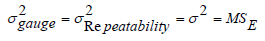
Finally, in order to validate the findings of the experiment, a gauge and measurement system capability study was done with the data points collected. Different gauge capabilities studies were utilized, as the implementation of these methods vary widely across the industry. The study thresholds selected for this research are commonly used for the different techniques. However, these thresholds can change depending on the requirements of the project [7]. In order to calculate most of the gauge capacity equations, the gauge variance. In order to calculate most of the gauge capacity equations, the gauge variance  must be found. Given that:


Because only one operator completed all the data collection of the within-subject design experiment with replicates, the reproducibility of the experiment is not being considered, just the repeatability. Therefore:
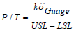
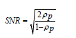
Consequently, the following equations were applied, and the results collected. Remember that all of these measurements are arbitrary and depend on the application, and the engineers responsible for determining what the threshold of the machine should be for a particular inspection process.
a) Precision-to-Tolerance (P/T) ratio: If P/T ≤1 adequate gauge capability can be (Table 8)
b) Measurement System Variability: Fraction of the total observed variance attributed to the machine (Table 9)
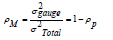
c) Processed Part Variability: Fraction of the total observed variance attributed to the part (Table 10)

d) Signal to Noise Ratio: If SNR ≥ 5 adequate gauge capability can be implied. An SNR ≤ 2 indicates inadequate capability (Table 11)
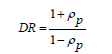
e) Discrimination Ratio: If DR ≥ 4 adequate gauge capability can be implied (Table 12
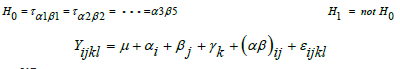
As expected, the studied CMM machine has a better resolution than both modalities in the CMA machine. As it can be seen in figure 8, the CMM measured flatness for 0° samples ranges from measurements close to 0.001in to no more than 0.003in, while the CMA contact and con-tactless recorded values range from almost 0.001in to about 0.006in, and from just below 0.004in to 0.006in respectively. These higher flatness values were expected, as the part without the surface cut (0°) had a rougher surface finish than the parts with the angled cuts. However, when we contrast the measured flatness for the parts with the machined surfaces (5°,10°), it can be seen that the CMM highest recorded value is below 0.001in for the 5° parts, while for the CMA contact modality, 0.001in is just about the minimum value recorded. Similar observations can be made when comparing the other provided tables for different degree/machine combinations. The number of points that the laser can capture does not appear to have an effect on the flatness value measured, because even though the number of points widely varied in each scan (Table 4), the recorded data for different replicates does not appear to be changing drastically as seen in figure 8 for FAROLP [8].


Figure 7 shows that the CMM data, while positively skewed, registered the majority of flatness measurements to be just around 0.001in (0.0012in). While the CMA with a probe is similarly on the positive skewed side and has a mean of just above 0.002in (0.0028in), and it contains the most outliers. In the case of the laser scan, the mean is just above 0.005in (0.0051in) and still positively skewed. Consequently, the contact modality in the CMA appears to perform slightly better than its contactless counterpart, but still not as good as the data recorded by the CMM [9].
In order to identify if there are significant differences between the CMM and CMA data re-cording modalities, we conducted a within-subject design ANOVA utilizing RStudio. ANOVA was selected to test the different variables of this experiment (machine type, degree cut, part number) and determine if they have any significant impact on the flatness values recorded. This investigation does not consider the effect of the operator, as only one individual performed the experiment. Therefore, our model is as follows:
Where
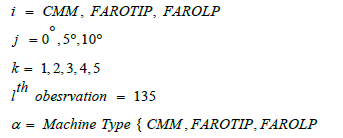
Our model compares machine, degree, and part, to test their impact on flatness. Because we are expecting to see differences on recorded flatness values between machine and degree, we have added the interaction effect between these two factors. In order to apply ANOVA, a test for normality was performed. The measured data was distributed as shown in figure 10. It can be seen that the data is skewed and does not follow a bell shape distribution. A Shapiro Wilk test proved that the data was not normally distributed. Therefore, we decided to transform the data by averaging the measured part flatness by machine and degree. This allowed us to have a single flatness value for each machine, degree, and part combination. The new table was used to conduct the ANOVA and checked for the distribution of the residuals, which showed that the data was normally distributed, as presented in figure 11. The Shapiro Wilk test of this data returned a p-value=0.95, therefore proving that the transformed data (in this case, the experimental error) is normally distributed. Hence, as established by the assumptions of ANOVA, we were able to utilize the model to conduct the test [10-13].
When applying the model to ANOVA, the result is that machine, degree, and their interaction, was significantly different (p-value<0.05). While part was not significantly different (p-value>0.05). To understand which elements of these factors are distinct, a Tukey test was completed. It was found that for the machines, the CMM is significantly different to the CMA contact and contactless method, while these two methods were significantly different from each other. In the case of the degrees, 0° was significantly different to 5°, and this one was significantly different to 10°. However, there were not significant differences between 0° and 10°. When looking at the differences in the interaction effects more closely, we can see that there are two main patterns. When the CMM machine is being considered with 0° against the other machined parts, there are significant differences, and this makes sense as the flatness values recorded by the CMM on the non-machined (original cold drawn surface) part were considerably higher than those from the machined parts. Moreover, other significant differences can be observed when comparing the CMM machine and CMA contact modality, against the CMA contact less modality. The flatness values recorded by the laser were substantially larger than the ones recorded by the other machines.
Now that we know all machines and some of the angles are statistically different when measuring flatness, we must determine what are the capabilities of each machine used. It can be seen from the data that all machines struggled when measuring the flatness of the 10° samples. The data points were more dispersed and the difference between the minimum and maximum values were higher than in any other combination of machine and degree. However, the Faro Laser Point performed poorly when looking at a part with that specific angle. That could be attributed to the way light from the laser might be reflecting from the material. Nevertheless, it is clear that across the different combinations, CMA contactless method did not have as good of a resolution as the CMA contact method and the CMM machine. The last two were close, but it is clear that for the measurements of 0°, 5°, and 10° cuts, the CMM was able to perform better than the CMA contact method.
In order to create a boundary which represents the usability of these machines (capacity to obtain the flatness we are trying to measure), we took three different approaches by utilizing the minimum, maximum and average flatness values recorded by the machines. If we would like to be conservative in the recommendations, we should select the maximum values presented in table 6. Meaning for example, that if we had a flatness tolerance of 0.004 in on a non-machined 0° cut aluminum surface, the CMM machine would be the only apparatus able to complete this task repeatedly, as all other options would not be capable of measuring that specific tolerance. For a more inclusive approach, the minimum values from table 7 will become the limiters of the operational range of the machine. However, the inherent risk is that the machine might not perform reliably to measure tolerances to what is needed. Therefore, a balanced approach will be utilizing the averages as illustrated in table 5. Averages will create boundaries where the machine has reliably obtained the data and allow the machines to be used in a wider range of tolerance levels, in turn making them more useful.
Lastly, for the gauge capability study calculations, we can see that when Precision-to-Tolerance is used, most machine-degree combinations are considered to have an adequate gauge capability in the experiment. Except, when the contact method of the CMA is being used for obtaining a tolerance of 0.0001in as the P/T values for that combination are larger than 0.1. When looking at the other measures, the combination of CMM with 10° pieces, and CMA contact with 10° pieces, have the highest percentage of observed contributed machine variance. This can be said, because when looking at the SNRs and DRs of calculated results of the aforementioned combinations, the results failed or were close to fail the given limits to evaluate adequate gauge capability. Meaning, that at those machine-degree combinations the gauge cannot be precise or accurate enough to be utilized in an inspection process regardless of its resolution. These analyses resulted in the different work envelopes (the range of flatness values that can be read by the machine on a specific configuration) shown on figure 12 below.
Conclusions and Recommendations
This study sees the CMM perform better than the CMA, because the CMM has a higher resolution; hence it is suggested to assign tasks to the machines based on the established capabilities discussed in this study. CMMs and CMAs have their own place in the manufacturing industry. Even though CMMs are better for metrology and feature verification regarding flatness, AA-CMMs such as the Faro Arm® are versatile and easier to use. It makes perfect sense for a shop to have either, or even better, both. Manufacturing environments are constantly evolving and working on different projects. So, depending on the working volume or tolerance level needed, these machines can be assigned to completely different tasks with the certainty that their performance will be appropriate for what is required.

To fulfill the goal of this pilot study, it is mentioned that a methodology and boundary must be created in order to provide the machinist or operators the opportunity to have a reference guide. This one will particularly guide workers and shops in selecting the appropriate tool for their metrology needs. Capabilities can be defined in different ways. We have highlighted three: conservative, inclusive, and balanced approach. It is recommended to utilize a balanced approach to guarantee that the machines are being utilized to their potential, while making sure not to push them beyond limits that will make the machine unreliable.
Therefore, regarding the boundary of the machines for flatness verification, we deter-mined that the CMM has a minimum measurable tolerance of 0.002in for 0° non-machined surfaces, 0.0006in for machined 5° surfaces, and 0.0009in for machined parts with 10° surface cut. The CMA contact has minimum measurable tolerance of 0.0032in for 0° non-machined surfaces, 0.0024in for machined parts with 5° surfaces cuts, and 0.0028in for 10° surfaces. Finally, the CMA contactless has minimum measurable tolerance of 0.0045in for 0° non-machined surfaces, 0.0045in for 5° surfaces, and 0.0063in for 10° surfaces. We have selected three overall boundaries that can be seen as the minimum tolerance the studied machines can handle, which can be used to easily assign tasks to the machines depending on the requirements of the project. The overall boundaries for flatness measurement are as follows:
a) CMM has a minimum measurable tolerance of 0.0006in
b) AA-CMM contact, has a minimum measurable tolerance of 0.0024in
c) AA-CMM contactless, has a minimum measurable tolerance of 0.0045in
It is clear from these observations and preliminary analysis that surface roughness and angles have an effect on the flatness data collected by the metrology devices studied. The gauge capability studies also showed that the machines were capable of measuring with precision certain combinations of machines and degrees, regardless of machine resolution. However, it can be concluded that some of the variance attributed to the machines, does not only relate to the machine itself, but to its operator. Based on those boundaries, the metrology device selection process is proposed in figure 12. An expanded version of these concepts can contain different setups for the two types of de-vices studied, other metrology devices, and brands. A database like this one could be applicable in determining machine shop capabilities for an integrative procurement system.

Future Research
As mentioned earlier, the operator error is inherent when utilizing an CMA. After experimenting, we can understand that an operator requires a certain level of experience and that, at the same time, taking measurements for prolonged periods of time can cause fatigue in the operator. Therefore, a similar experiment that accounts for user experience, or just multiple users, would be relevant, as we could quantify what part of the shortcomings in measuring with an CMA comes from the operator or operator experience.
On this experiment 70 points were taken from a 2.5 × 2.5in surface, which resulted on a point density of approximately 11 points per square inch. The effects of a part size increase should be studied, as it could become complicated having to collect twice as many points for a part twice as big. Understanding how many data points are needed based on surface size will directly impact the way in which we collect data, especially with CMA in contact modality. Understanding how the amount of surface data points collected affect the created Best Fit plane in order to analyze the required tolerances, is imperative as manufactured parts footprint keep increasing. Moreover, this research only studied one geometric form verification, flatness. It will be especially important to explore other geometric characteristics, like circularity or cylindricity, to expand the knowledge base methodology proposed in figure 12, including changes in probe size, materials, and other CMM or CMA device models (Figures 13 & 14).

Finally, this experiment was conducted utilizing a machined aluminum piece with no previous control values. To truly understand how far we are from the intended true value, repeating this experiment with a gauge or “perfect part” which was professionally manufactured and controlled, could help to properly identify the true differences between the CMM and AA-CMM methodologies studied.
References
- Groover M (2010) Fundamentals of Modern Manufacturing Materials, Processes, and Systems. In: (4th), John Wiley & Sons, Inc, USA.
- Kalpakjian S, Schmid S (2014) Manufacturing Engineering and Technology. In: (7th). Pearson, United Kingdom.
- Cuesta E, Gonzalez MD, Alvarez B, Barreiro J (2014) A new concept of feature-based gauge for coordinate measuring arm evaluation. IOP Science p. 25.
- Gupta N (2017) Factors Relevant to Parallelism Inspection. SHAREOK, USA.
- Kim W, Raman S (2000) On the selection of flatness measurement points in coordinate measuring machine in-spection. International Journal of Machine Tools and Manufacture 40(3): 427-443.
- Vijayarangan J (2017) Non-Contact Method to Assess the Surface Roughness of Metal Castings by 3D Laser Scanning, USA.
- Montgomery D (2013) Introduction to Statistical Quality Control. In: (7th), John Wiley & Sons, Inc, USA.
- Han S, Chunlong Z, Jianyu C, Shenghuai W (2021) Research on Micro/Nano Surface Flatness Evaluation Method Based on Improved Particle Swarm Optimization Algorithm. Frontiers in Bioengineering and Biotechnology 9: 775455.
- Lu J, Gao G, Yang H (2013) Error Modeling and Analysis of Articulated Arm Coordinate Measuring Machines. Advanced Materials Research pp. 464-467.
- Metrology Deals (n.d.). B&S MicroVal PFx 454 CMM.
- Acero R, Santolaria J, Bra A, Pueo M (2016) Virtual Distances Methodology as VerificationTechnique for AACMMs with a Capacitive SensorBased Indexed Metrology Platform. Sensors 16(11):1940.
- Lopez A (2019) Comparison of Discrete Part Verification Using Coordinate Measuring Machine and Articulated Arm Co-ordinate Measuring Machine. SHAREOK, USA.
- AAA Testers (n.d.). Faro Platinum 8FT FaroArm Portable CMM Measurement Inspection Arm.


