Research Article

Analysis of Environmental Prediction Data of Temperature and Relative Humidity from NCEP/NOAA

Ricardo Martins Campos¹* and Ronaldo Maia de Jesus Palmeira²

¹Centre for Marine Technology and Ocean Engineering (CENTEC), Instituto Superior Técnico, Universidade de Lisboa, Portugal

²Instituto de Astronomia, Geofísica e Ciências Atmosféricas (IAG), Universidade de São Paulo, Brazil

Submission: March 01, 2021;Published: March 17, 2021

*Corresponding author: Ricardo Martins Campos, Instituto Superior Técnico, University of Lisbon, Av. Rovisco Pais, 1049-001, Lisboa, Portugal

How to cite this article: Ricardo M C, Ronaldo M d J P. Analysis of Environmental Prediction Data of Temperature and Relative Humidity from NCEP/NOAA. Int J Environ Sci Nat Res. 2021; 27(4): 556217. DOI: 10.19080/IJESNR.2021.27.556217

Abstract

Environmental predictions have played an important role in our society in many different areas. Temperature and humidity are among the most important variables, being correlated with a number of human health problems, and deserve to be investigated. Therefore, our paper is dedicated to study the weather prediction data from the largest environmental agency that provides publicly-available global forecasts, the National Centers for Environmental Prediction (NCEP). Using 225 meteorological stations distributed worldwide, the operational forecast from NCEP is evaluated, with statistics applied to 5.397.315 pairs of forecasts and measurements. Our results indicate that 16-days forecasts have high accuracy but suffer from scatter errors that rapidly increase with longer forecast ranges. The root-mean-square (RMS) error for temperature is approximately 2°C to 3°C in the first four days of forecasts, and it reaches 6°C on the upper bound of the forecast range (16 days). The lowest RMS errors of relative humidity are also concentrated in the forecast range within the first five days, indicating larger errors beyond one week that are quantitatively analyzed in this paper.

Keywords: Weather forecasts; Environmental data assessment; Global forecast system; Biometeorology

Introduction

importance of weather forecasts relies on a variety of activities and users, including weather warnings to protect life and property, agriculture, management and planning of outdoor events etc. The association between meteorological conditions and human health is also an important aspect that has been widely studied. Royé et al. [1,2] indicated that apparent temperature [3] has a strong non-linear relationship with Ischemic Stroke and cardiovascular health. Associations between temperature and cardiovascular mortality have been reported by Basu et al. [4], while Alessandrini et al. [5] showed a strong relationship between biometeorological conditions and ambulance dispatches in Emilia–Romagna, Italy. Alessandrini et al. [5] found that ambulance dispatches increase 1.45% (non-traumatic diseases) and 2.74% (respiratory diseases) for every 1°C increase in the mean apparent temperature between 25° and 30°C. An overall increase of 0.9% in mortality per 1°C increase in AT was observed by Wichmann [6] and, more recently, Niu et al. [7] showed that low and high AT are significant risk factors of mental and behavioral disorders.

It is also well-known that environmental factors play an important part in the spread of certain virus diseases [8], most particularly for Influenza and other respiratory viral infections [9]. Previous studies indicate that low temperature and low humidity contribute to the increased risk of seasonal influenza [10-13]. Xiao et al. [14] and Zhang et al. [15] argue that the outbreak of influenza A (H1N1) had significant correlation with meteorological conditions. A similar relation for human rotavirus infection was described by Moe and Shirley [16], Brandt et al. [17], Konno et al. [18], Anestad [19], and Reyes et al. [20], with a stronger influence of temperature compared to humidity. Chan et al. [21] concluded that SARS coronavirus viability is lost at high temperatures above 38°C and high relative humidity above 95%, and Darniot et al. [22] similarly found that low temperatures influence human metapneumovirus (hMPV) and respiratory syncytial virus (RSV) activity.

Regarding the recent Coronavirus disease 2019 (COVID-19), Wang et al. [23] initially found that one-degree Celsius increase Abstract Environmental predictions have played an important role in our society in many different areas. Temperature and humidity are among the most important variables, being correlated with a number of human health problems, and deserve to be investigated. Therefore, our paper is dedicated to study the weather prediction data from the largest environmental agency that provides publicly-available global forecasts, the National Centers for Environmental Prediction (NCEP). Using 225 meteorological stations distributed worldwide, the operational forecast from NCEP is evaluated, with statistics applied to 5.397.315 pairs of forecasts and measurements. Our results indicate that 16-days forecasts have high accuracy but suffer from scatter errors that rapidly increase with longer forecast ranges. The root-mean-square (RMS) error for temperature is approximately 2°C to 3°C in the first four days of forecasts, and it reaches 6°C on the upper bound of the forecast range (16 days). The lowest RMS errors of relative humidity are also concentrated in the forecast range within the first five days, indicating larger errors beyond one week that are quantitatively analyzed in this paper. Keywords: Weather forecasts; Environmental data assessment; Global forecast system; Biometeorology in temperature and one percent increase in relative humidity lower daily effective reproductive number of COVID-19 by 0.0383 and 0.0224, respectively. In agreement with Wang et al. [23], the model results from Bannister-Tyrrell et al. [24] suggest a negative correlation in the predicted number of COVID-19 cases with temperature. Sajadi et al. [25] and Chen et al. [26] argued that including weather information it may be possible to improve models of community spread of COVID-19 in the future, allowing for concentration of public health efforts. However, numerical models used for weather forecasts are associated with high uncertainties and large errors [27-29] that must be carefully investigated.

Based on the vast variety of end uses to weather forecasts, we dedicate this work to evaluate the weather prediction data of selected environmental variables that most affect human lives. Our goal is to provide a valuable assessment of short- and midterm weather forecasts using a large number of quality-controlled meteorological stations.

Data and Methods

The environmental analysis is related to deterministic shortto mid-term forecasts, where the numerical weather prediction model (WP) is run every day with high resolution grid, fast assimilation of measurements, and with forecast range up to 16 days. The predictability of weather conditions is limited to a few days due to the chaotic behavior of the atmosphere. Lorenz (1963) [30] describe that skillful short-term weather forecasts have a fundamental limit of about two weeks.

The choice of relevant variables to be analyzed was based on previous studies of Wang et al. [23], Bukhari and Jameel [31], Sajadi et al. [25], Ishmatov [32], Royé et al. [1,2], Brini et al. [33], Sloan et al. [34], Wichmann [6], Zhang et al. [15], Lowen and John [35], Jaakkola et al. [12], Xiao et al. (2013) [14], Alessandrini et al. [5], Chan et al. [21], Żuk et al. [36], Lowen et al. [13], Konno et al. [18], & Moe and Shirley [16] – from where it has been selected air temperature at 2 meters height (T2M) and relative humidity (RH) as two important factors that affect human health in general.

The forecast data selected comes from the NCEP Global Forecast System (GFS) described by EMC (2003) - the best publicly-available global forecast, widely used worldwide. It is run every day, four times a day (cycles), out to 384 hours (16 days) with spatial resolution of 12 km and time resolution of 3 hours. Every cycle count with a robust data assimilation system that incorporates quality-controlled measurements to systematically improve the model initialization (“first-guess”) and consequently the whole forecast product. Yin et al. [37] and EMC (2003) provide more information about GFS. Yang et al. [27] evaluated the performance of GFS against observations made by the U.S. Department of Energy Atmospheric Radiation Measurement (ARM), focused on the surface energy fluxes and clouds. They obtained a good performance from GFS forecast that was able to capture the observed evolutions of cloud systems during major synoptic events. However, no inland recent assessment of T2M and RH has been available so far.

A new version of GFS (FV3, www.weather.gov/news/fv3) with improved physics and numerical scheme was put into operation in 06/2019 so the present assessment is based on GFS forecasts stored from 07/2019 to 03/2020 – approximately 8 months of data. The in-situ measurements selected for the GFS forecast assessment consist of surface observation data including inland meteorological stations, received via Global Telecommunications System (GTS), quality controlled and organized by the University Corporation for Atmospheric Research (UCAR). This research data archive (RDA/UCAR) is described by NCEP/NWS/NOAA [38]. The forecast and measurement data can be accessed at the links provided at the end of this paper.

The RDA/UCAR global database starts in 1999; however, the measurements for the forecast model assessments were obtained from 07/2019 until 03/2020 to be consistent with the new version of GFS forecast data, previously described. Thousands of stations are provided by RDA/UCAR all over the globe but the selection of proper data for comparison with GFS must be done with caution. The T2M and RH characteristics on the continent rapidly change in space whereas the grid resolution of GFS is 12km. For a reliable comparison of GFS with RDA/UCAR, interpolation should be avoided as well as stations distant from the model grid points. Hence, a sub-set of RDA/UCAR stations were selected with maximum distance to GFS grid points of 500 meters. Stations with many gaps and outliers were excluded. It leads to a total of 225 stations with latitude/longitude close to the nearest grid point of GFS, where the matchups could be directly built. Considering the period of 8 months over these stations, and the forecast range of 16 days (additional time dimension), the methodology resulted in 5.397.315 pairs of forecast/measurement utilized for the analyses and assessments.

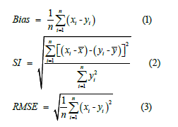
The statistical assessment was conceived to investigate accuracy and precision separately, being the accuracy related to the average deviation of the model predictions to the expected values, and precision related to the spread of such deviation – interpreted as systematic and scatter errors, respectively. Three error metrics were calculated, suggested by Campos et al. [39], to summarize the assessment (equations 1 to 3) where is the GFS forecast, is the measured data, and the overbar indicates the arithmetic mean. The Bias (equation 1) is associated with systematic errors, where positive values indicate that GFS overestimates the measurements and negative values that the measurement is greater than the forecast. The Scatter Index (SI) of equation (2) evaluates the scatter component of the error and it is always positive. The denominator of equation (2) indicates that the SI is normalized by the measurements and can be interpreted as ratios, or percentage errors when multiplied by 100. The Root Mean Square Error (RMSE) of equation (3) combines the systematic and scatter components of the error, being always positive. Additional guidance about forecast verification can be found at Jolliff et al. [40] and Ebert et al. [41].

Results

Equations (1) to (3) have been applied to the 5.397.315 matchups of GFS model forecasts with in-situ measurements covering 225 meteorological stations. From Table 1, the assessment shows underestimation of GFS compared to the stations, for both T2M and RH, i.e., the GFS forecast values are usually lower than the measurements, on average. This difference, associated with the systematic error, is very small, being less than 1°C in temperature. Moving to SI, the errors become much larger, where T2M presents 36% of scatter error and RH 20%. Looking at the Bias and SI together, we can conclude that GFS forecast model has a reasonably good accuracy but low precision. The overall forecast error, combined into the RMSE, shows T2M with 4.3°C and RH with 16.32%. The bulk error metrics presented by Table 1 selected the whole evaluation dataset, including different forecast lead times. It is intuitive that weather prediction tends to perform better at shorter ranges, e.g., for the same day or next 24 hours, than at longer leads around one week or more. Campos et al. [29,39] calculated the deterioration of weather predictions as a function of forecast time, which is intrinsic to the atmosphere chaotic nature described by Lorenz [30]. In light of this nature and to promote a more valuable assessment, the metrics are then recalculated for each forecast lead independently (Figure 1 & 2). The boxplots of Figure 1 summarize several aspects of the evolution of the error with the forecast range. The center marks of the boxes evolve through negative values, for RH and especially T2M, which indicate an increasing underestimation of GFS with longer forecast leads. These increasing systematic errors are small, with bias of T2M going to -2°C for the longest ranges. The boxplots also show the broadness of the error distribution, which indicates a large and increasing spread throughout the days. In the nowcast (beginning of the forecast) and in the first days, the spread is much smaller than the same error beyond one week. The rate of increasing of the scatter error is larger for T2M than RH. Nevertheless, the growth of scatter errors is common for both variables and it is quite significant.

The evolution of the SI with time is better illustrated in Figure 2. For T2M it starts with 0.23 and remains below 0.30 in the first six days. Beyond day-7, it rapidly increases to very large errors reaching 0.5 (same as scatter errors for T2M of 50% of the values) on day-15 and 16. For RH, the SI on the nowcast starts with 0.16 and follows a similar growing pattern until it reaches 0.23 (23% of scatter errors) after 13 days, when it stabilizes. The combination of scatter and systematic errors in the RMSE plots show smaller T2M errors below 3°C within the first four days, and larger errors above 5°C beyond ten days of forecast. The same RMSE for RH starts with 13% in the first day and it goes to 18% and above after ten days. The joint analysis of Figure 1 & 2 suggests a much better forecast skill in the first five days of forecasts that rapidly deteriorates with time, especially T2M. It also indicates that the greatest challenge in weather forecasting is to reduce scatter error at longer lead times.

Conclusion

In this paper we have discussed the quality of weather forecast data from NCEP. The forecast model was shown to have good accuracy but very large scatter errors that compromises the forecast precision. The deterioration of the forecast performance for longer forecast ranges is pronounced, as shown in Figure 1 & 2. Within the first four forecast days, the errors are relatively small with RMSE for T2M up to 3°C, whereas beyond 10 days the same RMSE is above 5°C. The RMSE for RH varies from 13% in the first forecast day to near 20% beyond 12 days. We can conclude that the performance of NCEP/GFS is mostly affected after the fifth day of forecast, and both T2M and RH from NCEP/GFS tend to be underestimated, i.e., the forecast usually provides lower temperature and humidity than the measurements. For the range of best forecast performance, within the first four days, the NCEP/ GFS errors of T2M varies from 2°C to 3°C and RH from 13% to 14%. Based on these results, end users should utilize weather forecast data with caution, considering the increasing errors with forecast time, and paying especial attention to large uncertainties beyond one week.

Acknowledgment

This study has been partially funded by the Research and Innovation Center (RIC) of AtmosMarine Ltda, www.atmosmarine. com. The authors would like to acknowledge the National Centers for Environmental Prediction (NCEP) and the Research Data Archive of the University Corporation for Atmospheric Research (RDA/UCAR) for providing the data.

Summary of Data Sources

NCEP’s Global Forecast System (GFS):

https://www.ftp.ncep.noaa.gov/data/nccf/com/gfs/prod/

Inland measurements from RDA/UCAR:

https://rda.ucar.edu/datasets/ds461.0/.

references

1. Royé D, Zarrabeitia MT, Riancho J, Santurtún A (2019a) A time series analysis of the relationship between apparent temperature, air pollutants and ischemic stroke in Madrid, Spain. Environmental Research 173: 349-358.
2. Royé D, Zarrabeitia MT, Arroyabe PF, Gutiérrez AA, Santurtú A (2019b) Role of Apparent Temperature and Air Pollutants in Hospital Admissions for Acute Myocardial Infarction in the North of Spain. Revista Española de Cardiología (English Edition) 72(8): 634-640.
3. Steadman RG (1984) A Universal Scale of Apparent Temperature. Journal of Climate and Applied Meteorology 23(12): 1674-1687.
4. Basu R, Wu X, Malig BJ, Broadwin R, Gold EB, et al. (2017) Estimating the associations of apparent temperature and inflammatory, hemostatic, and lipid markers in a cohort of midlife women. Environmental Research 152: 322-327.
5. Alessandrini E, Sajania SZ, Scotto F, Miglio R, Marchesi S, et al. (2011) Emergency ambulance dispatches and apparent temperature: A time series analysis in Emilia–Romagna, Italy. Environmental Research 111(8): 1192-1200.
6. Wichmann J (2017) Heat effects of ambient apparent temperature on all-cause mortality in Cape Town, Durban and Johannesburg, South Africa: 2006-2010. Science of The Total Environment 587-588: 266-272.
7. Niu Y, Gao Y, Yang J, Qi L, Xue T, et al. (2020) Short-term effect of apparent temperature on daily emergency visits for mental and behavioral disorders in Beijing, China: A time-series study. Science of the Total Environment 733: 139040.
8. Hemmes JH, Winklers KC, Kool SM (1962) Virus Survival as a Seasonal Factor in Influenza and Poliomyelitis. Antonie van Leeuwenhoek 28: 221-233.
9. Minhaz SM, Dean Ud (2010) Structural explanation for the effect of humidity on persistence of airborne virus: Seasonality of influenza. Journal of Theoretical Biology 264(3): 822-829.
10. Tsuchihashi Y, Yorifuji T, Takao S, Suzuki E, Mori S. et al. (2011) Environmental factors and seasonal influenza onset in Okayama city, Japan: case-crossover study. Acta Med Okayama 65(2): 97-103.
11. Shaman J, Pitzer VE, Viboud C, Grenfell BT, Lipsitch M (2010) Absolute humidity and the seasonal onset of influenza in the continental United States. PLoS Biol 8(2): e1000316.
12. Jaakkola K, Saukkoriipi A, Jokelainen J, Juvonen R, Kauppila J, et al. (2014) Decline in temperature and humidity increases the occurrence of influenza in cold climate. Environ Health 13(1): 22.
13. Lowen AC, Mubareka S, Steel J, Palese P (2007) Influenza virus transmission is dependent on relative humidity and temperature. PLoS Pathogens 3(10): 1470-1476.
14. Xiao H, Tian HY, Lin XL, et al. (2013) Influence of extreme weather and meteorological anomalies on outbreaks of influenza A (H1N1). Chin Sci Bull 58(7): 741-749.
15. Zhang Y, Feng C, Ma C, Yang P, Tang S, et al. (2015) The impact of temperature and humidity measures on influenza A (H7N9) outbreaks—evidence from China. International Journal of Infectious Diseases 30: 122-124.
16. Moe K, Shirley JA (1982) The Effects of Relative humidity and Temperature on the Survival of Human Rotavirus in Faeces. Archives of Virology 72(3): 179-186.
17. Brandt CD, Kim HW, Rodriguez WJ, Arrobio Jo, Jeffries BC, et al. (1982) Rotavirus gastroenteritis and weather. J Clin Microbiol 16(3): 478-482.
18. Konno T, Suzukt H, Katsushirna N, Imai A, Tazawa F, et al. (1983) Influence of temperature and relative humidity on human rotavirus infection in Japan. J Infect Dis 147(1): 125-128.
19. Anestad G (1987) Surveillance of respiratory viral infections by rapid immunofluorescence diagnosis, with emphasis on virus interference. Epidemiol Inf 99(2): 523-531.
20. Reyes M, Eriksson M, Bennet R, Hedlund WO, Ehrnst A (1997) Regular pattern of respiratory syncytial virus and rotavirus infections and relation to weather in Stockholm, 1984-1993. Clinical Microbiology and Infection 3(6): 640-646.
21. Chan KH, Peiris JSM, Lam SY, Poon LLM, Yuen KY, et al. (2011) The Effects of Temperature and Relative Humidity on the Viability of the SARS Coronavirus. Advances in Virology 2011(734690).
22. Darniot M, Pitoiset C, Millière L, Aho Glélé LS, Florentin E, et al. (2018) Different meteorological parameters influence metapneumovirus and respiratory syncytial virus activity. Journal of Clinical Virology 104: 77-82.
23. Wang J, Tang K, Feng K, Lv W (2020) High Temperature and High Humidity Reduce the Transmission of COVID-19. BMJ Open Forthcoming.
24. Tyrrell MB, Meyer A, Faverjon C, Cameron A (2020) Preliminary evidence that higher temperatures are associated with lower incidence of COVID-19, for cases reported globally up to 29th February 2020.
25. Sajadi MM, Habibzadeh P, Vintzileos A, Shokouhi S, Wilhelm FM, et al. (2020) Temperature, Humidity and Latitude Analysis to Predict Potential Spread and Seasonality for COVID-19.
26. Chen B, Liang H, Yuan X, Hu Y, Xu M, et al. (2020) Roles of meteorological conditions in COVID-19 transmission on a worldwide scale. MedRxiv.
27. Yang F, Pan HL, Krueger SK, Moorthi S, Lord SJ (2006) Evaluation of the NCEP Global Forecast System at the ARM SGP Site. Monthly Weather Review 134(12): 3668-3690.
28. Wang W, Chen M, Kumar A (2010) An Assessment of the CFS Real-Time Seasonal Forecasts. Weather. Forecast 25(3): 950-969.
29. Campos RM, Alves JHGM, Penny SG, Krasnopolsky V (2020) Global assessments of the NCEP Ensemble Forecast System using altimeter data. Ocean Dynamics 70: 405-419.
30. Lorenz EN (1963) Deterministic nonperiodic flow. J Atmos Sci 20(2): 131-141.
31. Bukhari Q, Jameel Y (2020) Will coronavirus pandemic diminish by summer?
32. Ishmatov A (2020) Influence of weather and seasonal variations in temperature and humidity on supersaturation and enhanced deposition of submicron aerosols in the human respiratory tract. Atmospheric Environment 223: 117226.
33. Brini I, Bhiri S, Ijaz M, Bouguila J, Merchaoui SN, et al. (2018) Temporal and climate characteristics of respiratory syncytial virus bronchiolitis in neonates and children in Sousse, Tunisia, during a 13-year surveillance. Environmental Science and Pollution Research 27(19): 23379-23389.
34. Sloan C, Heaton M, Kang S, Berrett C, Wu P, et al. (2017) The impact of temperature and relative humidity on spatiotemporal patterns of infant bronchiolitis epidemics in the contiguous United States. Health & Place 45: 46-54.
35. Lowen A, John S (2014) Roles of humidity and temperature in shaping influenza seasonality. J Virol 88(14): 7692-7695.
36. Żuk T, Rakowski F, Radomski JP (2009) Probabilistic model of influenza virus transmissibility at various temperature and humidity conditions. Computational Biology and Chemistry 33(4): 339-343.
37. Yin J, Hain CR, Zhan X, Dong J, Ek M (2019) Improvements in the forecasts of near-surface variables in the Global Forecast System (GFS) via assimilating ASCAT soil moisture retrievals. Journal of Hydrology 578: 124018.
38. National Centers for Environmental Prediction/National Weather Service/NOAA/U.S. Department of Commerce (2004) NCEP ADP Global Surface Observational Weather Data, October 1999 – continuing. Research Data Archive at the National Center for Atmospheric Research, Computational and Information Systems Laboratory, Boulder CO.
39. Campos RM, Alves JHGM, Penny SG, Krasnopolsky V (2018) Assessments of surface winds and waves from the NCEP Ensemble Forecast System. Weather and Forecasting 33(6): 1533-1564.
40. Jolliff JK, Kindle JC, Shulman I, Penta B, Friedrichs MAM, et al. (2009) Summary diagrams for coupled hydrodynamic-ecosystem model skill assessment. Journal of Marine Systems 76(1-2): 64-82.
41. Ebert E, Wilson L, Weigel A, Mittermaier M, Nurmi P, et al. (2013) Progress and challenges in forecast verification. Meteorol Appl 20(2): 130-139.