Research Article

Developing Climate Change Projections using Different Representative Concentration Pathways of Emission Scenario: In the Case Jimma, Ethiopia

Moges Molla*

Ethiopian Environment and Forest Research Institute, Ethiopia

Submission: August 14, 2020; Published: September 16, 2020

*Corresponding author: Moges Molla, Ethiopian Environment and Forest Research Institute, Hawassa Center, Hawassa, Ethiopia

How to cite this article: Moges M. Developing Climate Change Projections using Different Representative Concentration Pathways of Emission Scenario:In the Case Jimma, Ethiopia. Int J Environ Sci Nat Res. 2020; 25(3): 556175. DOI:10.19080/IJESNR.2020.26.556175

Abstract

Anthropogenic influence on the climate system is clear, and the recent emissions of greenhouse gases are the highest in history. This particular activity is aimed to project the future climate using different representative concentration pathways of emission scenarios for Jima station. Statistical downscaling approach was used to downscale rainfall and temperature. Predictors were synthesized based on correlation analysis between large scale climate predictors and observed station climate data. Monthly predictors were used to establish a regression model between the predictors and observed climate variables. The regression models were validated against observed station data and were used to generate downscaled future rainfall and temperature. Data for future scenario were collected from the Canadian Centre for Climate Modeling and Analysis (CCCma) of Canada Environment. The minimum temperature will be increased from 0.50C to 0.80C from the lowest to worst emission scenario for neat term period and 1.20C to 2.60C for end of century respectively. Similarly the maximum temperature will be increased 1.20C to 2.00C for near term century and 2.30C to 3.90C for midterm and 3.70C to 4.70C for end of century under RCP2.6, RCP4.5 and RCP8.5 which alarming mitigation measures. There is low % of precipitation change or increasing depends on RCPs the Projection changes slight increase in precipitation for main rain seasons (AMJ) and (JAS) is only under RCP2.6 but there is decrease under RCP4.5 and RCP8.5 for all time horizon of 2020’s, 2050’s and 2080’s. The projected change in annual mean temperature under RCP2.6 (upper), RCP4.5 (middle) and RCP8.5 (bottom) scenarios: approximately 3.7°C, 4.2°C and 3.7°C respectively.

Keywords: Emission; Scenario; RCPs; Projection

Introduction

Climate change can be defined as a change in the state of the climate that can be identified by changes in the average and/or the variability of its properties, and persist for an extended period of time, normally a decade or longer stated [1]. The impact of changing climate, such as rising global average temperatures and increases in frequency and severity of extreme events, droughts and floods, are already affecting human being, biodiversity and ecosystems, economies and societies worldwide [2]. Seasons are shifting, temperatures are climbing and sea levels are rising around the globe. Meanwhile, our planet must still supply us and all living things with air, water, food and safe places to live.

Human influence on the climate system is clear, and recent anthropogenic emissions of greenhouse gases are the highest in history. Recent climate changes have had widespread impacts on human and natural systems. Warming of the climate system is unequivocal, and since the 1950s, many of the observed changes are unprecedented over decades to millennia. The atmosphere and ocean have warmed, the amounts of snow and ice have diminished, and sea level has risen. The globally averaged combined land and ocean surface temperature data as calculated by a linear trend show a warming of 0.85 [0.65 to 1.06]°C, over the period 1880 to 2012, for which multiple independently produced datasets exist. The total increase between the average of the 1850-1900 period and the 2003-2012 period is 0.78 [0.72 to 0.85]°C, based on the single longest dataset available. For the longest period when calculation of regional trends is sufficiently complete (1901 to 2012), almost the entire globe has experienced surface warming IPCC, Climate Change 2014 Synthesis Report [3].

Climate change in ethiopia

At recent decade, the problem of climate variability and climate change, due to anthropogenic as well as natural processes, has come with daily bad news [4]. Ethiopia is vulnerable to the impacts of climate change and the unpredictability of climate variability. The country’s adaptive capacity is constrained by limited livelihood options for the majority of the population, inadequate ability to withstand or absorb disasters and the prevailing biophysical shocks it faces [5]. Drought, rain fall delay, fire damage and heavy and unexpected rain fall are climate related hazards that mainly faced and also total crop loss, reduced yield, reduced seeding quality, delayed maturity and increased crop pest/disease are the major climate impacts, [6]. Climate change is expected to have adverse ecological, social and economic impacts. Quantitative climate change impact assessments made so far on various socioeconomic sectors are limited in the country. According to [7], an increased precipitation over Ethiopia is projected during the 21st century, except the negative to no change projections of the RCP2.6 over the eastern part of the country. The ensemble-mean annual precipitation for all RCPs increase by 4% to 12% by 2100 compared to the 1975- 2005 baseline. The response of different parts of the country to different RCPs is slightly different. The percentage increase is high over northern part of Ethiopia under RCP2.6 scenario and over southern and east-southern part of the country under RCP4.5 and RCP8.5 scenarios.

Although there is a slight spatial difference among the three RCPs in mean temperature projections of the 2020s, the difference increases with time. The range of annual temperature increase for all the RCPs by 2100 relative to the 1975-2005 baseline period mean ranges from -0.5° to 6°C. Under RCP2.6 the mean temperature increases by approximately 1°C at the end of the century relative to the baseline period, and 5°C in RCP8.5. For RCP 4.5, which represents the moderate scenario, the projected increase in temperature is around 2°C. According to Ethiopian panel on Climate Change First Assessment Report, Working Group I Physical Science Basis [5]. The EPCC projections indicate temperatures increases from -0.5° to 6°C 2100 relative to the 1975-2005 baseline period for all the RCPs. the projected change in annual mean temperature under RCP2.6 (upper), RCP4.5 (middle) and RCP8.5 (bottom) scenarios: approximately 1°C, 2°C and 5°C, respectively 33 [5].

Climate change scenarios for Africa, based on the results from several General Circulation Models using the data collected by the Intergovernmental Panel on Climate Change Data Distribution Centre (IPCC-DDC) indicate that future warming across Africa ranges from 2oC (low scenario) to 5oC (high scenario) by 2100. Therefore, the result obtained from SDSM lies within the range of IPCC recommendations [3].

The representative concentration pathway scenarios (RCP)

The representative concentration pathways (RCP) are the latest generation of scenarios that provide input to climate models. Scenarios have long been used by planners and decision makers to analyze situations in which outcomes are uncertain. In climate research, emissions scenarios are used to explore how much humans could contribute to future climate change given uncertainties in factors such as population growth, economic development, and development of new technologies. Projections and scenarios of future social and environmental conditions are also used to explore how much impact lesser or greater amounts of climate change would have on different possible states of the world, for example futures with greater or lesser amounts of poverty. The purpose of using scenarios is not to predict the future, but to explore both the scientific and real‐world implications of different plausible futures [8].

Over time, a variety of approaches to scenarios in climate research have been used, from stylized representations of annual percentage increases in global average concentrations of greenhouse gases to advanced representations of emissions of many gases and particles affecting climate and derived from detailed socioeconomic and technology assumptions.

Downscaling methods and tools

The general circulation models (GCMs) used to simulate and project future climate with forcing by greenhouse gases and aerosols, typically dived the atmosphere and ocean in to horizontal grid with a resolution of 2o latitude by 4o longitude, with 10 to 20 layers in the vertical. In general, most GCMs simulate global and continental scale processes in detail and provide a reasonable accurate representation of the average planetary climate. Over the past decade, the sophistication of such model has increased and their ability to simulate present and past global and continental scale climate has substantially improved. Nevertheless, while GCM demonstrates significant skill at the continental and hemispherical scale and incorporate a large portion of the complexity of the global system, they are inherently unable to represent local subgrid scale features and dynamics, such as local topographical feature and convective cloud process [9]. Moreover, GCM were not designed for climate change impact studies and do not provide a direct estimation of the hydrological response to climate change. For example, assessment of future river flow may require (subscenarios) daily precipitation in the catchment even at station scales. Therefore, there is a need to convert GCM out put into at least a reliable daily rainfall series at the scale of the watershed to which the hydrological impact is going to be investigated. The method used to covert GCM output into local meteorological variables required for reliable hydrological modeling are usually referred to as downscaling techniques. There are two categories of climate downscaling methods namely dynamic downscaling and statistical downscaling [9].

Statistical downscaling

Empirical downscaling starts with the premise that the regional climate is the result of interplay of the overall atmospheric or oceanic circulation as well as of regional topography, land-sea distribution and land use. As such empirical downscaling seeks to drive the local scale information from the larger scale through inference from the cross-scale relationship using some random or deterministic functions. In most cases, the regional climate is seen as random process conditioned up on a driving large scale climate regime. Therefore, the confidence that may be placed in downscaled climate change information is foremost dependent on the validity of the large –scale field from GCM. For instance, derived variables (not fundamental to the GCM physics but derived from the physics) such as precipitation are usually not robust information at the regional and local scale [10]. Conversely, tropospheric quantities like temperature or geo-potential height are intrinsic parameters of the GCM physics and are more skillfully represented by GCM.

Finally, climate change projections which can indicate temperature nature and precipitation patterns in the 2020’s, 2050, and 2080’s timeframe, can be used to guide major investment decisions relating to long-term water management, such as when and where to build new water reservoirs. Effective climate services need to exploit the full potential of existing knowledge and new research developments. However, though the understanding of the climate system is advancing quickly, it is not being used effectively in development planning and practice in area. This study aimed to improve climate information services by providing specific point location projection using different representative concentration emission climate scenarios for near term, midterm and end of century time horizon.

Objective of study

To develop climate change scenario for Jimma station under high, medium and low representative concentration pathways (RCPs).

Materials and Methods

Research design

have been developed to simulate the present climate and have been used to predict future climatic change but GCM are at high resolution and there need to be downscale the results from such models to individual sites or localities for impact studies using SDSM. Atmospheric large scale variables (CanESM2 Predictors) will be downloaded from IPCC’s Fifth Assessment Report (AR5) CMIP5/ Coupled Model Inter-comparison Project, Phase 5 (CMIP5)/ a collaborative climate modeling process coordinated by the World Climate Research Programme (WCRP). The second generation of Earth System Model CanESM2 is the fourth generation coupled global climate model developed by the Canadian Centre for Climate Modelling and Analysis (CCCma) of Environment Canada. http://climate-scenarios.canada. ca/?page=pred-canesm2.

SDSM description

SDSM permits the spatial downscaling of daily predictorpredictand relationships using multiple linear regression techniques. The predictor variables provide daily information concerning the large-scale state of the atmosphere, whilst the predictand describes conditions at the site scale.

There are only few meteorological stations specially in developing countries particularly in Ethiopia that have no complete and fully accurate time series weather data. Hence, filling of missed and incorrect recorded measured data was controlled prior to application for this practical situations. The first step before model calibration was quality control using SDSM through identification of gross data errors, missing data codes and outliers to get the appropriate quality data.

The screening Predictor a variable was be done by trial and error procedure for model calibration. Using the partial correlations statistics, predictors which showed the strongest association with the predictand were selected. Assembly and calibration of statistical downscaling model(s) - the large-scale predictor variables identified are used in the determination of multiple linear regression relationships between these variables and the local station data. Then SDSM manual procedure was be followed to generate climate scenario for the basins [11].

Data sources

Observed daily precipitation and maximum and minimum temperatures data was obtained from weather stations located in or near the watershed. National Centre for Environmental Prediction (NCEP) data was generated for missing data filling and GCM-derived predictors will be generated form global data base. Climate data downscaled using SDSM was analyzed for trend test analysis of projected rainfall and temperature was done using Man Kandell.

SDSM modeling approach

The downscaling of the GCMs data using SDSM was done following the procedures in use manual. Before starting the main SDSM downscaling operation, quality control of the data was undertaken to check the input data file for missing and unreasonable values. Scatter plot analysis was performed and it was checked that all the predictands were normally distributed; hence transformation operation was found unimportant for unconditional process. The other operations performed for downscaling are dealt in detail in the following sections.

The SDSM software reduces the task of statistically downscaling daily weather series into seven discrete steps: Quality control and data transformation; Screening of predictor variables; Model calibration; Weather generation (using observed predictors); Statistical analyses; Scenario generation [11].

Setting of the model parameter

Year length: The normal calendar year (366 days) which allows 29 days in February every fourth year was used whenever dealing with predictand and NCEP predictor whereas the year length of 360 days was used in the scenario generation part since CanESM2 data uses model years consisting of 360 days as follows according to [11].

Event Threshold: The event threshold is set to 0.05 for temperature and 0.1 mm/day for precipitation to treat trace rain days as dry days.

a) Model Transformation: The model transformation is applied to the predictand in conditional models. The default (None) is used for the predictand that is normally distributed as in the case of daily temperature and fourth root transformation is applied for precipitation since the model is conditional and the data is skewed.

b) Variance inflation: Variance inflation controls the magnitude of variance inflation in the downscaled daily weather variables. This parameter can be adjusted during the calibration period to force the model replicate the observed data. The default value (i.e.12) produces approximately normal variance inflation prior to any transformation and is applied to maximum and minimum temperature. For precipitation this parameter can be adjusted during the calibration period and was set to 16 [11]. c) Bias correction: Bias correction compensates for any tendency to over or underestimates the mean of the conditional process by the downscaling model. This parameter is set to1 (default value) for maximum and minimum temperature since the process is non-conditional whereas for precipitation this parameter can be adjusted in order to match the mean of the conditional process and is set to 0.95 [11].

Downscaling the GCM for the baseline period

The base line scenarios downscaled for base period for Jimma station using 30-years daily data from 1988-2018 was selected to represent baseline for this study. Thus, the CanESM2 was downscaled for the baseline period for the three representative concentration pathway scenarios and the statistical properties of the downscaled data was compared with observed data. The downscaling experiment was conducted for minimum temperature; maximum temperature and precipitation based on the data from NMA for the above stations which contain observed data for the specified period and the results are discussed in section below.

Results and Discussion

Calibration and validation

The calibration was carried out from 1988-2003 for fifteen years and the withheld data from 2004-2018 were used for model verification. The model develops a better multiple regression equation parameters for the maximum and minimum temperature than the precipitation. This Result is mainly due to the conditional nature of precipitation. In conditional models, there is an intermediate process between regional forcing and local weather (e.g., local precipitation amounts depend on wet-/ dry-day occurrence, which in turn depend on regional-scale predictors such as humidity and atmospheric pressure) [11].

Minimum temperature

The monthly minimum temperature downscaled for NCEP in the baseline period for Jimma meteorological station is shown in Figure 1.

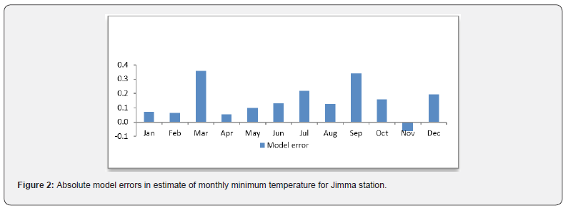
The result of downscaling minimum temperature indicates that there is very good agreement between observed and simulated minimum temperature. As shown in Figure 2: it was also found that, during the month of Jan, Feb and April the model error is very small. However, during the month of Mar and Sep the model error is 0.35oC and 0.341oC in addition to that during the month of Nov the model underestimates. The model error in each month is less than the projected temperature change in the future.

Maximum temperature

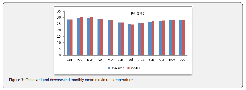
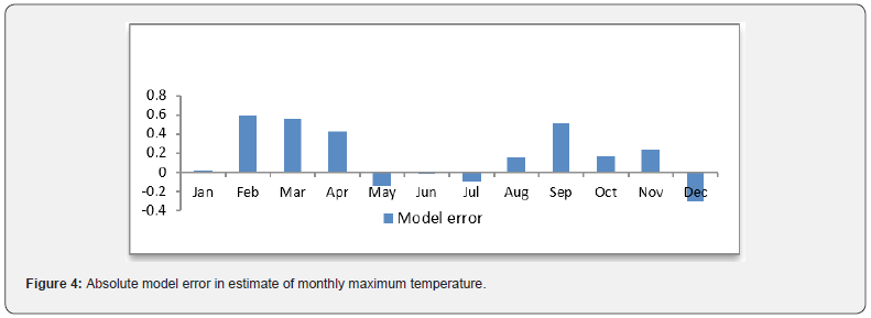
The monthly maximum temperature downscaled for NCEP in the baseline period is shown in Figure 3. The result of downscaling maximum temperature indicates that there is an excellent agreement between observed and simulated maximum temperature. However as shown in Figure 4 the model underestimates maximum temperature during the month Dec and overestimates on Feb, Mar, April ,Sep and Nov but during the remaining months, the model error is negligible.

Precipitation

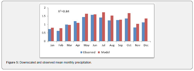
Relative to the minimum and maximum temperature the precipitation could not be able to replicate the historical (observed) data. This is due to complicated nature of precipitation processes and its distribution in space and time. Climate model simulation of precipitation has improved over time but is still a problematic [12], also added that rainfall predictions have a larger degree of uncertainty than that of temperature. This is because rainfall is highly variable in space and so the relatively coarse spatial resolution of the current generation of climate models is not adequate to fully capture that variability. However, the RS value is 0.84 shown in Figure 5 below.

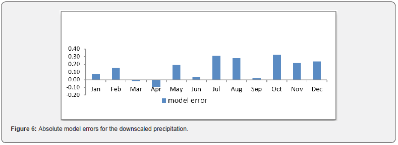
The downscaled precipitation shows an average absolute model error of 0.31mm and 0.33mm for the month of Jul and Oct respectively however the error is negligible for the month of Mar, Jun and Sep respectively in Figure 6 below.

Anomalies of Climate variable under different RCPs emission scenarios

Minimum temperature anomaly

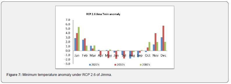
Anomaly: is a departure from a reference value or long-term average. As Figure 7 shown below a positive anomaly indicates that the observed temperature was warmer than the long- term mean under RCP2.6 for most of months and decrease for months AMJJAS in 2050’s time horizon.

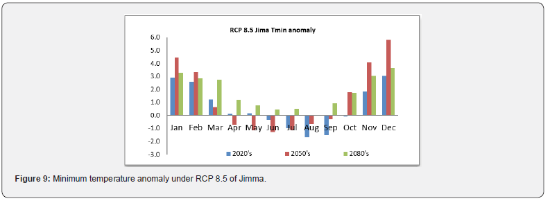
Under RCP 4.5 and RCP 8.5 Figure 8 & 9 below shows that the main rain seasons has negative anomaly which means the observed minimum temperature is cooler than the long mean average minimum temperature. Unlikely observed minimum temperature warmer for months ONDJFM under both scenarios.

Maximum temperature anomaly

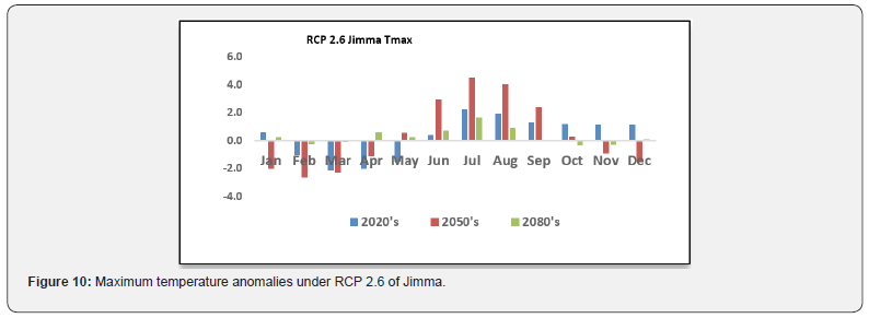
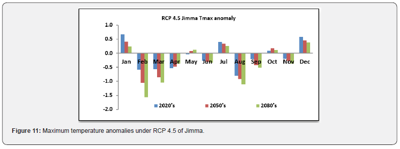
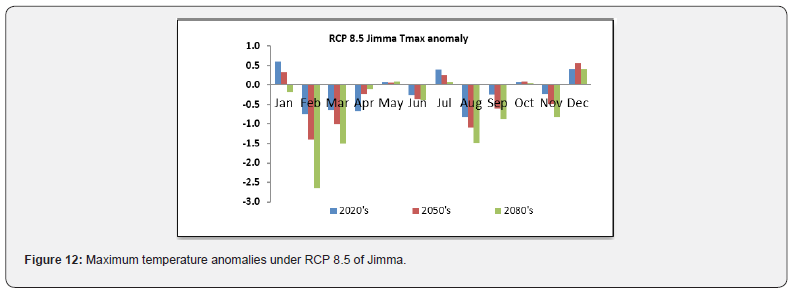
In Figure 10-12 below the maximum temperature anomaly seems differnet from that of minimum temperature. Under RCP 2.6 among the main rain season months like JJAS shows positive anomaly for all three time horizones (2020’s, 2050’s and 2080’s). Similarly, for months OND the maximum temperature has positive anomaly for 2020’s only but negative for november and december.

As Figure 11 & 12 indicated under RCPs 4.5 and 8.5 the maximum temperature anomaly seem similar for some months but in Figure 11 only months JMJO and D has positive anomaly for all time horizon similarly in Figure 12 also.

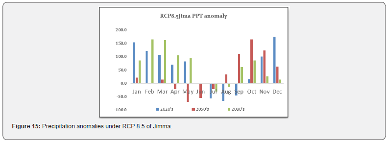
Precipitation anomaly

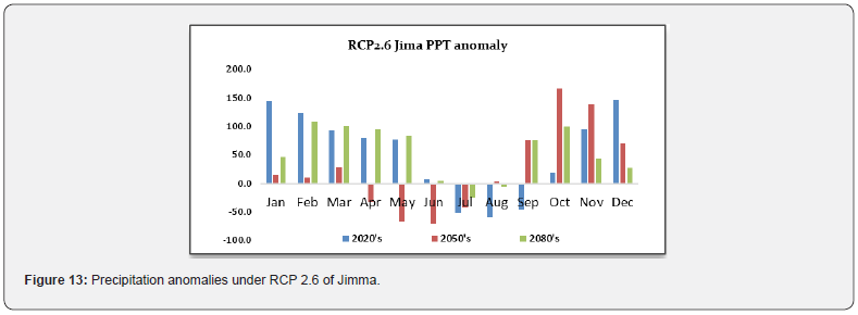
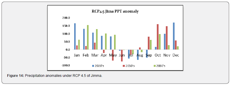
a) Positive anomaly: indicates where precipitation was above the long-term normal. The mean annual rain fall will increase and more rain will occur for most of dry months.

b) Negative anomaly: indicates where precipitation was below normal. The main rainy months MAM and JJAS becoming below normal as emission level increase (Figure 13-15).

Projected future climate variables / scenario generation

After the calibration and validation of SDSM model, carried out, the daily future climate variables are projected for the next century using the CanESM2 Global Circulation Model. The projection generates 20 ensembles of daily climate variables, which are equally plausible; hence, these ensembles were averaged out in order to consider the characteristics of all those 20 ensembles. With the aid of statistical downscaling model, the GCMs global predictors were used for development of future climate scenarios and the analysis was made for 2020s, 2050s and 2080s for RCP2.6,RCP4.5 and RCP8.5 representative concentration path way scenarios.

Minimum temperature

The downscaled minimum temperature shows an increasing trend in all future time horizons for RCP2.6, RCP4.5 and RCP8.5 scenarios for the stations. The downscaled minimum temperature in 2020’s indicated that the minimum temperature would rise by 0.50C, for RCP2.6 scenarios. For the same time horizon under RCP4.5 scenario the minimum temperature will rise by 0.60C.

In the case of RCP8.5 it will increased respectively. In 2050s the increment will be 0.80C, 10C and 2.90C under RCP2.6 RCP4.5 and RCP8.5 scenario. The increment will be expected to be high in 2080s, which is 1.20C for RCP2.6 scenario 1.80C for RCP4.5 scenarios and finally 2.60C rise in minimum temperature will be expected under RCP8.5 scenario.

Maximum temperature

Similar to projected average monthly minimum temperature, maximum temperature also reflects increasing trend in future climate periods. The projected maximum temperature in 2020s for Jimma station indicated that maximum temperature would rise by 1.20C respectively for RCP2.6 similarly by 1.50C for RCP4.5 and for the worst scenario RCP8.5 by 2.10C. In 2050s the increment will be 2.30C under RCP2.6, 2.90C under RCP4.5 and 3.90C under RCP8.5 scenarios for the station. In 2080s the maximum temperature will be increased by 3.70C RCP2.6 scenario. Under RCP4.5 scenario the maximum temperature will be increased by 4.20C. For the last scenario RCP8.5 the future maximum temperature will rise by 4.70C. This shows that the future period will experience increasing trend in maximum temperature for both the three representative pathway scenarios. However, the increments will be less for RCP2.6 scenario relative to RCP8.5 scenario.

Precipitation

The projected mean annual precipitation in 2020s for station were indicated that mean annual precipitation will decrease by 7.4% under RCP2.6 similarly by 7%, under RCP4.5 and for the worst scenario RCP8.5 by 7.5%. In 2050s the decrement will be 8% under RCP2.6, 8 %under RCP4.5 and 8.2 under RCP8.5 scenarios for the station. In 2080s the projected precipitation will be decreased by 7.7% under RCP2.6 scenario. Under RCP4.5 scenario it will be decreased by 8%, 10% and 5.6%. For the last scenario RCP8.5 the future precipitation will be expected to decrease by 8.5%. Overall, the three scenarios of CanESM2 projected a diminishing trend in the annual precipitation for specific station.

Conclusion and Recommendation

The minimum temperature will be increased from 0.50C to 0.80C from lowest emission scenario to the worst emission scenario for neat term period and 1.20C to 2.60C for end of century. Similarly the maximum temperature will be increased 1.20C to 2.00C for near term century and 2.30C to 3.90C for midterm and 3.70C to 4.70C for end of century under 2.6, 4.5 and 8.5 RCPs which require mitigation activities.

There is low % of precipitation change and or increasing depending on RCPs but there will be significant increasing with in different time horizon of 2020’s, 2050’s and 2080’s but for mainly rain months there will be the decreasing of rf happened on near term and end of century under RCP2.6 and RCP 8.5.

The study revealed that the Rf increase/ decrease varies depending the season/months/period /scenario’s and time horizon the average annual rainfall will increase by 5.8%, 5.9% and 6.3% for rcp 2.6, 4.5 and 8.5 scenarios respectively for near term and similarly for mid-term but decease for the end of century.

references

1. USAID (2007) A Guidance Manual for Development Planning: Adapting to Climate Variability and Challenge United states.
2. UNEP (2006)&US EPA (2016) Overview of Greenhouse Gases.
3. IPCCs AR5 Working Group 3 Report released in March 2014. Shared socioeconomic pathways (SSPs).
4. Molla M (2016)Prediction of Future climate and its Impact on Crop Production and possible adaptation Strategy. SNNPR Shashogo woreda, Ethiopian Environments and Forest Research Institute Hawassa Center, Ethiopia.
5. NAPA-ETH (2019) Climate Resilient Green Economy (CRGE); Ethiopia National Adaptation Plan (NAP-ETH) climate change in the country development policy framework.
6. Molla M (2016)Climate Variability, its impact on Maize Production and Adaptation options: Case Study of Halaba Special Woreda,Southern. Ethiopian Environments and Forest Research Institute Hawassa Center, Ethiopia.
7. NAPA (2007)National Meteorological Service Agency of Ethiopia. Climate Change National Adaptation Programme ofAction (NAPA) of Ethiopia. Addis Ababa, Ethiopia.
8. Moss RH,Edmonds JA, Hibbard KA, Manning MR, Rose SK, et al.(2010) The next generation of scenarios for climate change research and assessment. Nature 463: 747-756.
9. DibikeYB, CoulibalyP(2005)Hydrologic impact of climate change in Saguenay watershed: comparison of downscaling methods and hydrologic models. Journal of Hydrology 307(1-4): 145-163.
10. CuderlikJM(2007)Hydrologic models for inverse climate change impact Modeling ,the 18^th Canadian Hydrological Conference on Challenges for water resource Engineering in a changing world,Manitoba, August 22-24,2007.
11. Wilby Robert L, Christian W Dawson (2007) Using SDSM Version 4.1 SDSM 4.2.2 - A decision support tool for the assessment of regional climate change impacts, User Manual, Leics, LE11 3TU, UK.
12. Bates et al. (2008) Climate Change and Water. Technical Paper of the Intergovernmental Panel on Climate Change, IPCC Secretariat, Geneva, p. 210.