Research Article

Implementation of Deep Learning and Machine Learning Algorithms for Predicting the Stress Intensity Factor (KI) in Cracked Mechanical Components Deep Learning for Stress Intensity Factor Prediction

Manuel Nazario Rocha-Martínez^1,2*, Guillermo Urriolagoitia-Sosa¹*, Beatriz Romero-Ángeles¹, Reyner Iván Yparrea-Arreola^1,2, Cyntia Iurhuari Garcia-Felix², Blanca Estela Verdin-Gutierrez², Josué Sebastián Aviña-Gonzalez², Iván Alejandro López-Zumaran^1,2, Félix de Jesús Mar-Luna^1,2 and Francisco Carrasco-Hernandez²

¹Instituto Politécnico Nacional, Escuela Superior de Ingeniería Mecánica y Eléctrica, Sección de Estudios de Posgrado e Investigación, Unidad Profesional Adolfo López Mateos “Zacatenco”, Col. Lindavista, Alc. Gustavo A. Madero, CP 07320, Ciudad de México

²Universidad Tecnológica de Durango, Departamento Académico de Ingeniería en Mantenimiento Industrial, Carretera Durango-Mezquital, km 4.5 S/N, Gavino Santillán, Durango C.P. 34308, México

Submission: March 13,2025;Published:March 24,2025

*Corresponding author:Manuel Nazario Rocha-Martínez, Guillermo Urriolagoitia-Sosa, Instituto Politécnico Nacional, Escuela Superior de Ingeniería Mecánica y Eléctrica, Sección de Estudios de Posgrado e Investigación, Unidad Profesional Adolfo López Mateos “Zacatenco”, Col. Lindavista, Alc. Gustavo A. Madero, CP 07320, Ciudad de México, Email: mrocham2201@alumno.ipn.mx, gurriolagoitias@ipn.mx.

How to cite this article:Manuel Nazario Rocha-M, Guillermo Urriolagoitia-S, Beatriz Romero-Á, Reyner Iván Yparrea-A, Cyntia Iurhuari Garcia-F. Implementation of Deep Learning and Machine Learning Algorithms for Predicting the Stress Intensity Factor (KI) in Cracked Mechanical Components Deep Learning for Stress Intensity Factor Prediction. Eng Technol Open Acc 2025; 6(3): 555688.DOI: 10.19080/ETOAJ.2025.06.555688

Abstract

In Fracture Mechanics, predicting the stress intensity factor (SIF, Mode I, K_I) is crucial, as it enables the assessment of a component’s resistance in the presence of cracks and, consequently, the prevention of catastrophic failures. The correlational study between machine learning (ML) and deep learning (DL) methodologies allowed us to demonstrate that crack length is closely related to SIF. However, the primary focus was to evaluate both methodologies and achieve a more precise prediction of KI. To this end, a numerical analysis was conducted using the finite element method (FEM), considering as a case study the cross-section of a square metallic plate with a central crack. This analysis was performed using ANSYS Mechanical APDL, which also facilitated the generation of a robust database containing crack size values and their corresponding K_I. The intelligent algorithms were developed in Python and executed on the Jupyter Notebook platform. Prior to the implementation of ML and DL, an exploratory data analysis (EDA) was conducted to gain a better understanding of the dataset’s characteristics.

Keywords:ANSYS; Stress; Exploratory; Jupyter; Deep Learning; Machine Learning Method

Abbreviations:SIF: Stress Intensity Factor; ML: Machine Learning; DL: Deep Learning; FEM: Finite Element Method; EDA: Exploratory Data Analysis; SVR: Support Vector Regression; ELU: Exponential Linear Unit

Introduction

Currently, the relationship between the Mode I Stress Intensity Factor (KI) and the length of a mechanical crack (a) is a key aspect in evaluating mechanical components. This relationship is based on Griffith’s theory and the linear elastic fracture model, which establish that, from a dimensional approach, the stress intensity factor should be linearly related to the applied stress and the square root of the crack length [1,2]. Understanding this relationship is essential for predicting the failure behaviour of materials under stress. The objective of this research is to determine the degree of correlation between KI and crack length, based on the widely accepted notion in the mechanical literature t hat there is a direct and strong link between these two variables, as well as modelling through deep learning and machine learning techniques to predict KI [3]. Given this, it is understandable that this correlation is critical in industrial sectors such as aerospace, civil engineering, and mechanical engineering, as the structural integrity of the materials used is a decisive factor [4]. A square metallic plate with a central crack was used as a case study. The plate underwent a symmetric numerical analysis to determine the stress intensity factor at the crack tip, where the finite element method analysis was performed on the same geometry with variations of 0.1 mm in the crack size (starting from the crack tip) to generate the necessary database for training the two intelligent methodologies (ML and DL).

Materials and Methods

Theoretical Background

In fracture mechanics, a mathematical expression allows us to determine the Stress Intensity Factor (SIF) in a typical manner. For this analysis, Mode I (opening or tensile), one of the three relative types of motion between the two fracture surfaces, was used. This equation is given by [5]:

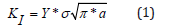
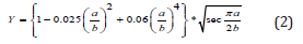
Where K_I corresponds to the stress intensity factor, Y is the applied geometry factor (dependent on the crack), σ is the applied stress, and a is the crack length. In this research, Tada’s formula was used for the analytical evaluation of a circular plate with a central crack. Below is the geometric variant within Tada’s formula [5].

Finite element method analysis

For this study, a square geometry of 200mm x 200mm was used, under numerical simulation conditions with symmetry (aiming to optimize computational resources). A static, isotropic, and homogeneous analysis was performed, assuming the Young’s modulus of steel (200 GPa). For the analysis, Equation (1) was used in conjunction with Equation (2). The discretization at the crack was implemented using the KSCON command with a radius of 0.5mm and a division of 12 elements at the crack tip, all done in a controlled manner to obtain stress concentration. The loading conditions were 200 MPa with a symmetric simulation in both X and Y directions to work with a quarter of the component. A new working plane, CS 11, was implemented, where a nodal analysis of 3 nodes was conducted [6] to determine the KI factor for different crack origin increments, with variations of 0.1mm in the range of 1 to 20mm, discarding minimum crack values of 1mm. Consequently, the K_I values were generated using the KCALC command. The relationship between KI and crack length, both analytically and numerically, can be visualized in (Figure 1) [6,7].

(Figure 2) shows the result of the nominal stress analysis concentrated at the crack tip by applying boundary conditions and load. The distribution of concentrated stress was observed, representing the critical area where crack propagation is expected to occur. The areas of highest concentration identified the regions with the greatest risk of structural failure, providing key information about the material’s integrity, which is essential for predicting the component’s behavior [8].

The comparison of results obtained from the finite plate analysis using the Finite Element Method (FEM) with ANSYS APDL showed a high degree of agreement with theoretical values. It can be concluded that as the crack length decreases (approaching 1 mm), the percentage of error between the analytical and numerical results diminishes. In contrast, as the crack length increases beyond this value, the error difference between the analytical and numerical results grows. In this analysis, 192 elements were chosen to assess the impact of increasing crack length, shown in (Figure 3) [9].

Exploratory Data Analysis (EDA)

The foundation of this study lies in the data analysis, which summarizes the main characteristics observed within the dataset. Understanding these aspects is crucial before applying any predictive or inferential modeling techniques involving machine learning. To achieve this, an analysis of dimensions, data types, statistical data types, correlation between variables and constants, and the relationship between crack size and stress intensity factor was conducted [10]. Among these aspects, the primary focus was placed on the fourth stage, where the direction and intensity of the linear relationship force between pairs of variables is determined. To achieve this, in (Figure 4), I show the resulting graph, where it can be noted that some variable names are in our native language, Spanish, because all the variables code are written in Spanish and for practical and coding purposes, I have chosen to leave them in this format, just for clarification [11].

For this study, variables, and constants such as Young’s modulus, Poisson’s coefficient, geometry width, and applied stress were integrated. In the main diagonal, the elements are one, which is expected since each variable is perfectly correlated with itself. In other words, stress intensity factor and crack size coincident with themselves. Moving away from the diagonal to notable values, the factor r = 0.9517556 is observed. There is a strong positive correlation between crack size (tam_grieta) and stress intensity factor (factor_intensidad). This indicates that as the crack size increases, the stress intensity factor also tends to increase linearly [12].

Machine learning method

For this, the SVR (Support Vector Regression) algorithm was used as an initial phase in Machine Learning, enabling the correlation and analysis of the data [13]. It is an extension of Support Vector Machines (SVM), and this modeling is particularly useful when the problems being analyzed do not exhibit a linear trend. To reach this conclusion, a machine learning algorithm was implemented and trained using a dataset of two hundred values (crack size and stress intensity factor), applied to square geometries. Similarly, linear regression, ridge regression, lasso, Bayesian ridge, and finally Support Vector Regression (SVR) [14] algorithms were used to identify the best algorithm that could predict the stress intensity factor with the highest accuracy, all these shown in the (Figure 5).

We can observe how the SVR algorithm is the one that most closely approximates the natural response of the evolution of the stress intensity factor values, corresponding a Pearson correlation analysis [15].

Deep Learning Method

In this process, a multilayer perceptron [16] neural network was implemented, which defines a neural network model using Keras [17], a deep learning library in Python commonly used with TensorFlow. The neural network defined in the code has a sequential structure, meaning that the layers are stacked one after another. First, a sequential model called ‘K1-Predictor’ is created, which stacks the layers linearly, and the network is trained so that the output of one layer is the input to the next. In the first layer, there is no weight; it only specifies the input data format [18]. In this case, it means that the model expects an input with a single feature (i.e., a one-dimensional vector of size 1). Specifically, this layer takes a single value as input at each step of the model. The first hidden layer of the model has 150 neurons and uses the ELU (Exponential Linear Unit) activation function, which is a nonlinear function that allows us to improve performance and training speed [19]. The second hidden layer of the model has fifty neurons and again uses the ELU activation function. This reduces the number of neurons from 150 to 50, which is common in deep networks to refine information as it progresses through the layers. Finally, the output layer of the model has only one neuron because the network is expected to make a prediction of a single value (such as a regression) [20]. No activation function is specified for this layer because, by default, the output will be a linear value (ideal for regression).

The previously defined neural network model was trained using the training dataset x_train and y_train, where the chosen validation parameter was 20%, meaning that 20% of the training data would be used for model validation during the training process. The model was trained for 80 epochs, meaning that the data would pass through the network eighty times to adjust the weights [21]. The training progress, including detailed information for each epoch, was displayed, and the input data was randomly shuffled before each epoch, helping to prevent overfitting and improving the model’s generalization. The training analysis results were shown in the (Figure 6) [22].

Results

Through the application of machine learning and deep learning methodologies, values with a high accuracy index were obtained when comparing the analytical, numerical, and predicted values through both approaches. This is evident in (Table 1), which displays selected values for different crack sizes, along with their corresponding results from the Tada formula, finite element analysis, and machine learning predictions.

On the other hand, we can see the results of the application of the deep learning method, in (Figure 7), as well as in (Table 2).

Conclusion

This study established the correlation of the stress intensity factor (K_I) as a function of crack size (analytically and numerically), yielding highly satisfactory results. Using programming tools in Python and Jupyter, the correlation index was graphically represented, supporting the assertions made by many authors in fracture mechanics, where KI is shown to have a linear and directly proportional relationship with crack size. Furthermore, the interpolation technique prediction demonstrated remarkable accuracy, closely matching the numerical and analytical K_I values, which highlights the potential of using machine learning and deep learning techniques as complementary tools in fracture mechanic’s research. The application of these techniques not only optimizes the time spent on designing and numerically analyzing mechanical components but also reduces the complexity associated with lengthy modelling processes. It is important to emphasize that, rather than replacing traditional numerical modelling methods such as the Finite Element Method (FEM), machine learning adds value by effectively complementing these approaches. These tools allow for faster and more accurate predictions, enriching and streamlining the analysis processes without compromising the rigor of evaluating the results. In summary, combining numerical techniques and artificial intelligence opens new opportunities to improve efficiency and accuracy in studying stress intensity factors, representing a valuable innovation in fracture mechanics.

Acknowledgements

The authors gratefully acknowledge the Instituto Politécnico Nacional, Universidad Tecnológica de Durango and Consejo Nacional de Humanidades Ciencias y Tecnologías for supporting this research.

Conflict of Interest

The authors declare no conflict of interest.

References

1. Rodríguez Villarreal O (2017) Scaling Exponents in Fracture Surfaces of Granular Composites. Master's Thesis, Universidad Autónoma de Nuevo León, pp 23-24.
2. Urriolagoitia Sosa G (1996) Application of Fracture Mechanics to the Case of Cracked Structures Under Fatigue Loads. Master's Thesis, SEPI ESIME Zacatenco, Instituto Politécnico Nacional.
3. Broberg KB (1968) Critical review of some theories in fracture mechanics. International Journal of Fracture Mechanics 4: 11-18.
4. Gdoutos EE (2012) Fracture Mechanics Criteria and Applications. Springer Dordrecht, Netherlands, pp. 314.
5. Tada H (1971) A note the finite width corrections to the stress intensity factor. Engineering Fracture Mechanics 3(3): 345-347.
6. Hernández Gómez LH, Urriolagoitia Calderón G, Urriolagoitia Sosa G (2009) Assessment of the structural integrity of cracked cylindrical geometries applying the EVTUBAG program. Technical Journal of the Faculty of Engineering, University of Zulia 32(3): 190-199
7. Urriolagoitia Sosa G, Romero Angeles B, Hernández Gómez LH, Torres Torres C, Urriolagoitia Calderón G (2011) Crack-compliance method for assessing residual stress due to loading/unloading history: Numerical and experimental analysis. Theoretical and Applied Fracture Mechanics 56(3): 188-199.
8. Esparragoza IE (1998) Crack Tip Stress Study for Elastic-Perfectly Plastic Materials with Some Applications. Tesis doctoral, Florida International University.
9. Irwin GR (1957) Analysis of stresses and strains near the end of crack traversing a plate. Journal of Applied Mechanics 24(3): 361-364.
10. Velasco MC, Zhao I (2021) Descriptive statistics; An introduction to univariate and bivariate exploratory data analysis, Metro Ciencia 29(3): 53-62.
11. Rodríguez AS (1984) Some Considerations on the Use of Pearson's r Coefficient as an Index of Agreement Between Observers. Mexican Journal of Behavior Analysis 10(2): 137-160.
12. Fiallos G (2021) Pearson Correlation and the Regression Process Using the Least Squares Method. Ciencia Latina; Multidisciplinary Journal 5(3): pp. 1-19.
13. Möller DPF (2019) Machine learning and deep learning. Guide to Cybersecurity in Digital Transformation, Springer Cham, Switzerland, 347-384.
14. Goddard-Close J, de los Cobos-Silva SG, Pérez-Salvador BR, Gutierrez-Andrade MA (2000) An Algorithm for Training Support Vector Machines for Regression. Journal of Mathematics; Theory and Applications 7(1-2): 107-116.
15. Chicco D, Warrens MJY, Jurman G (2021) The coefficient of determination R-squared is more informative than SMAPE, MAE, MAPE, MSE and RMSE in regression analysis evaluation. Peer Journal of Computer Science 7: 1-24.
16. Brownlee J (2022) How to Build Multi-Layer Perceptron Neural Network Models with Keras. Machine Learning Mastery.
17. Brownlee J (2018) Deep Learning with Python: Develop Deep Learning Models on Theano and Tensor Flow Using Keras. Machine Learning Mastery, 1-64.
18. Abadi M, Barham P, Chen J, Chen Z, Davis A, et al. (2016) TensorFlow: A System for Large-Scale Machine Learning. In 12th USENIX Symposium on Operating Systems Design and Implementation, Savannah, GA, USA, 265-283.
19. Clevert DA, UnterthinerT, Hochreiter YS (2016) Fast and Accurate Deep Network Learning by Exponential Linear Units (ELUs).
20. Barba R, Mantilla C, Arellano A, Ramos V, Barrazueta P, et al. (2019) Application of Multilayer Perceptron in Traffic Prediction for Academic and Enterprise Networks. Infociencia 12: 633-648.
21. Hecht-Nielsen R (1989) Theory of the backpropagation neural network. Neural Networks for Perception 1: 593-605.
22. Galvañ Sala DA (2021) Comparison of Techniques for Overfitting Prevention in Neural Networks. University of Alicante, Spain.