


Comparative Analysis of Initial Feasible Solutions to Balanced Transportation Problems
Collins O Akeremale*1, 2, Faith Anthony1 and Segun Olaiju2
1 Department of Mathematical Sciences, Federal University Lafia, Nigeria
2 Deparment of Mathematical Sciences, University Technology, Malaysia
Submission: October 01, 2019; Published: October 29, 2019
*Corresponding author:Collins O Akeremale, Department of Mathematical Sciences, Federal University Lafia, Nigeria. Department of Mathematical Sciences, University Technology, Malaysia
How to cite this article:Collins O Akeremale, Faith Anthony, Segun Olaiju. Comparative Analysis of Initial Feasible Solutions to Balanced Transportation Problems. Eng Technol Open Acc. 2019; 3(2): 555607. DOI: 10.19080/ETOAJ.2019.03.555607
Abstract
In this work, we compared three transportation approaches to find the most efficient transportation schedule and the best transportation route for the initial feasible solution in order to maximize profit. Excel solver as a tool was used to compute the optimal solution as a validation for the optimal test.
Keywords:Transportation cost; Transportation problem; Initial basics feasible solution; Excel solver; Optimal solution
Introduction
One of the important applications of linear programming is in transportation problems. Transportation problem is a classical class optimization problem which involves moving goods from one location to another location depending on demand and supply of the goods at the various locations. Hitchcock [1] originally developed transportation problems and Dantzig [2] successfully developed efficient and robust method for the solution of the problems followed by Cooper & Henderson [3] who later improved on the method of solution.
The simplified version of simplex method is transportation method and it can be used to solve linear programming problems. It is known as the transportation problem/model because in solving problems that involves several sources and destinations, transportation method is a major application. A transportation problem is said to be balanced if, total supply equals total demand, if there is a disparity between demand and supply, it is said to be unbalanced transportation problem. In this work, we will focus on balanced transportation problems
Many authors [4-11] had worked on transportation problems with most of them laying emphasis on Vogel approximation method and northwest corner rule method for both the initial basic feasible solution and optimal solution. Though their results were found to be very good but, in this research, we intend to explore row minimal, column minimal and least square methods to obtain both the initial basic feasible solution and the optimal solution for possible comparison.
Problem Formulation
A firm produces goods at locations, i.e. 1,2,3, , im=…. The supply product at thi location = si, the demand for the goods is spread out at different demand locations i.e. 1,2,3, ,.jn=… The demand at the thj demand location is jD. The problem of the firm is to get goods from supply locations to demand locations at minimum cost. Assume that the cost of shipping one unit from supply location to demand location j is ijc and that shipping cost is linear, which means that if you shipped xij unit from location to demand location, then, the cost would be cijxij.
Where xij is the number of units shipped from supply location i to demand location j the problem is to identify the minimum or maximum shipping cost schedule. The constraints being that supply must meet demand at each demand location and cannot exceed supply at each supply location.
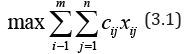
By the assumption of linearity, the schedule cost is as below
The total amount shipped out of supply location is
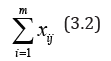
i.e. xij is the unit shipped from i to j. Also, from amount of unit can be shipped to any demand location 1,2,3, ,.jn=… The quantity cannot exceed the supply available, hence the constraint
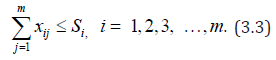
Similarly, the constraints that guarantee that the demand at each demand location is met is given by

Thus, we assume that the total supply is equal to total demand that is if
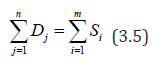
The constraints in the problem holds as equations
With the establishment that total supply is equal to total demand, the standard transportation model formulation is given below with the objective to find a transportation plan denoted by ij x that satisfy (3.5) and solves

In the problem it is natural to assume that the variable ij x takes on integer value (and non-negative ones). That is one can only ship items in whole number batches.
Then the standard mathematical model for this problem is:
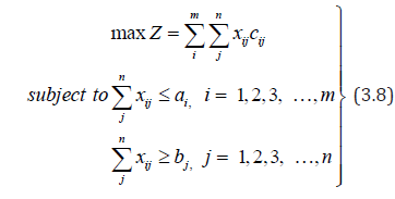
where
m = number of sources
n = number of destinations
i a =capacity of ith source
j b =capacity of jth destination
ij c = cost coefficient for materials shipped from ith source to jth destination
ij x =amount of materials shipped between ith source to jth destination
Methodology
In this section, we consider column minima, row minima and least square methods for the initial feasible solution of balanced transportation problems while we improve on each of the method for the optimality solution. The basic steps involved in solving a transportation problem are;
(i) find an initial basic feasible solution,
(ii) test the solution for optimality
(iii) improve the solution when it is not optimal at the initial feasible point.
In a case where the solution is not optimal at the initial feasible solution, steps (ii) and (iii) are repeated until an optimal solution is arrived at. Excel solver was also used for the optimality test.
Data collection and analysis
Data for this research work were collected from Pleasure Travels Limited, Peace Mass Transit, Blue Whales Transport Limited and Young Shall Grow Transport Limited and used for comparison of transportation algorithm(s) with the view of finding the most efficient transportation algorithm and the best transportation route for the benefit of the companies involved in order to maximise profit. Three methods of finding initial feasible solution (Column minima method, Row minima method and Least cost method) where employed. Excel solver was used to compute the optimal solution as a validation tool for the transportation problem.
Construction of pleasure travels transportation table
Consider a transportation company Pleasure Travels that allocates buses to different route on a daily basis and the total income generated on each per trip (to-fro) as well as the total passengers transported per trip (to-fro) as shown in (Table 1) below is transformed into transportation tableau and the initial feasible solution of the transportation problem is computed as follows (Table 2).


Now, we compute the total number of passengers that uses bus A to all the routes from Abuja Demand = 28+72+42+42 = 184
Total number of passengers that uses bus B to all the routes Demand = 28+72+42+42 =184
Total number of passengers that uses bus C to all the routes from Abuja
Demand = 26+26+72+26 = 150
Total Demand = 518
Number of passengers that moved from Abuja to Calabar using bus A to D = 82
Number of passengers that moved from Abuja to Owerri using bus A to D = 170
Number of passengers that moved from Abuja to Lagos using bus A to D = 156
Number of passengers that moved from Abuja to Ibadan using bus A to D = 110
Total supply = 82+170+156+110 = 518. This gives a balanced transportation problem hence; it satisfies the condition Total
Demand = Total SupplyTotal income generated is calculated below
6800 * 56 = ₦380,800
6600 * 26 = ₦171,600
7100 * 144 = ₦1,022,400
7000 * 26 = ₦182,000
6500 * 84 = ₦546,000
6400 * 72 = ₦460,800
5800 * 84 = ₦487,200
5400 * 26 = ₦140,400
Total income = ₦3,391,200
Finding initial feasible solution
Column minima method
The initial basic feasible solution is obtained using column minima method following the algorithm presented starting from the least cell in the first column until all demand and supply are met as shown in (Table 3).
Total income generated by the column minima method
6800 * 82 = ₦557,600
7100 * 20 = ₦142,000
7000 * 150 = ₦ 1,050,000
6500 * 102 = ₦663,000
6500 * 54 = ₦351,000
5800*110= ₦638,000
Total income = ₦3,401,600

Row minima method
The Row Minima Method is applied starting allocation to the cell with the minimum cost in the first row following the algorithm mentioned earlier as shown in (Table 4).

Total income generated using the Row Minima Method
6600 * 82 = ₦541,200
7000 * 68 = ₦476,000
7100 * 102 = ₦724,200
6500 * 156 = ₦1,014,000
5800 * 28 = ₦162,400
5800 * 82 = ₦475,600
TOTAL INCOME = ₦3,393,400
Least cost method
The initial basic feasible solution is obtained using the least cost method following the algorithm presented earlier starting from the least cell until all demand and supply are met as shown in (Table 5).

Total income generated using the least cost method is calculated below
6800 * 82 = ₦557,600
7100 * 20 = ₦142,000
7000 * 150 = ₦1,050,000
6500 * 82 = ₦533,000
6500 * 74 = ₦481,000
5800 * 110 = ₦638,000
Total income =3,401,600
Construction of Peace Mass Transit Transportation Problem
(Table 6) is transformed into a transportation tableau and the initial feasible solution of the transportation problem is computed as follows (Table 7).


Column minima method
Total income generated by the column minima method (Table 8)
6700 * 104 = ₦698,800
6600 * 4 = ₦26,400
6000 * 106 = ₦ 636,000
7000 * 98 = ₦686,000
5600 * 8 = ₦44,800
5600 * 74 = ₦414,400
5600*54 = ₦302,400
Total income = ₦2,806,800
The row minima method
Total income generated using the row minima method (Table 9).
Total income generated using the least cost method (Table 10).
6700 * 104 = ₦696,800
6700 * 4 = ₦26,800
6000 * 106 = ₦636,000
7000 * 98 = ₦686,000
5600 * 4 = ₦22,400
5600 * 78 = ₦436,800
5600 * 54 = ₦302,400
Total income = ₦2,807,200
Construction of blue whale’s transport company limited transportation problem
(Table 11) above can be transformed into transportation tableau as shown in the next table (Table 12).


Column minima method
Total income generated using the column minima method (Table 13).
5750 * 132 = ₦759,000
5300 * 84 = ₦445,200
7600 * 128 = ₦972,800
6600 * 80 = ₦528,000
6600 * 88 = ₦580,800
6600 * 36 = ₦237,600
5300 * 36 = ₦190,800
Total income = ₦3,714,200

Row minima method
Total income generated using the row minima method (Table 14).
5750 * 132 = ₦759,000
5300 * 84 = ₦445,200
5200 * 36 = ₦187,200
7600 * 128 = ₦972,800
6600 * 44 = ₦290,400
6600 * 88 = ₦580,800
6600 * 72 = ₦475,200
Total income = ₦3,701,600

The least cost method
Total income generated using the least cost method (Table 15).
5750 * 88 = ₦506,000
5750 * 44 = ₦253,000
5300 * 120 = ₦636,000
7600 * 96 = ₦72,960
7600 * 32 = ₦243,200
6600 * 176 = ₦1,161,600
6600 * 28 = ₦184,800
Total income = ₦3,714,200

Construction of young shall grow transportation table
(Table 16) above can be transformed into transportation tableau as shown in the next table (Table 17).


Column minima method
Total income generated using the column minima method (Table 18).
4600 * 176 = ₦809,600
4600 * 56 = ₦257,600
4200 * 176= ₦739,200
4100 * 112 = ₦459,200
5300 * 144 = ₦763,200
5000 * 132 = ₦660,000
5000 * 56 = ₦280,000
Total income = ₦3,968,800

The row minima method
Total income generated using row minima method (Table 19)
.4600 * 176 = ₦809,600
4600 * 56 = ₦257,600
4200 * 176= ₦739,200
4100 * 112 = ₦459,200
5300 * 132 = ₦699,600
5300 * 12 = ₦63,600
5000 * 188 = ₦940,000
Total income = ₦3,968,800

The least cost method
Total income generated using least cost method (Table 20).
4600 * 120= ₦552,000
4600 * 112 = ₦515,200
4200 * 176= ₦739,200
4200 * 112 = ₦470,400
5300 * 132 = ₦699,600
5300 * 12 = ₦63,600
5000 * 188 = ₦940,000
Total income = ₦3,980,000

Result
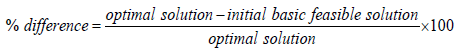
Using the excel solver application, the optimal solution for the four companies were obtained as follows: Pleasure Travels Limited = N 3,401,600, Peace Mass Transit = N2,823,600, Blue Whales Transport Company Limited = N 3,714,200, Young Shall Grow Motors Limited = N 3,980,000. The table below shows the companies name, initial income generated by the companies, the initial basic feasible solution using the three (3) different methods of solving transportation problems, the optimal solution obtained using the excel solver, the difference between the optimal solution and the initial basic feasible solution methods and the percentage (%) difference (Table 21).
Difference = Optimal Solution – Initial Basic Feasible Solution
From the table above it is clear that the column minima method generated the same income as that of the optimal solution for two companies (Pleasure Travels and Blue whales Travels), and generated income less than that of the optimal solution for two companies (Peace Mass Transit and Young Shall Grow Motors Limited). However, the column minima method generates a higher income than the initial income for all the companies. The row minima method generated an income the same as the optimal solution for none of the companies. However, the row minima method also generates a higher income than the initial income for all the companies.

The least cost method yields the best initial basic feasible solution for all the companies as its income generated were found to be the same as that of optimal solution for three companies (Pleasure Travels, Blue whales Transport Company and Young Shall Grow Motors Limited) and generates an income less than that of the optimal solution for one company (Peace Mass Transit). This could be achieved because it takes into consideration the least cost associated with each route alternatives. Although it takes a longer time to compute, this is something the Column Minima Method and Row Minima Method could not have achieved.
The above data is shown graphically in (Figures 1-3).


Conclusion
An advantage of the transportation problem algorithm is that, the solution process involves only main variables, artificial variables are not required as in the case of simplex method. Large transportation problem could relatively be solved using the transportation algorithm. It was shown that solving balanced transportation problem was easier using the column minima method and row minima method using the transportation problem formulated for Pleasure Travels, Bluewhales Transport Co. Ltd, Peace Mass Transit and Young Shall Grow Motors Ltd. The least cost method was found to be a bit difficult to calculate, yet it always yields a better result near optimal if not optimal. It can therefore be concluded that the least cost method although not quite as easy as the other methods, facilitates a better initial basic feasible solution than the column minima method and the row minima method. The optimal solution obtained using the excel solver application for the four (4) companies were found to be N3,401,600.00, N3,714,000.00, N2,823,600.00 and N3,980,000.00 respectively. It should be noted that although the Least cost method facilitates an optimal or near optimal result, it is not too reliable since it did not yield an optimal result for all the companies.
Recommendation
The use of a scientific approach gives a systematic and transparent solution as compared with a haphazard method. Using the more scientific assignment problem model for a given transportation problem gives a better result and management may benefit from the proposed approach to guarantee optimal profits from them. We therefore recommend that the assignment problem model should be adopted by managements of transportation companies for maximum profits. In general, the passenger population (demand) is always greater than the vehicle availability (supply). But this can only be verified (for an unbalanced transportation problem), if the actual data management and records are always available for researches to be carried out on them. Further research needs to be carried out in the area of bus services and maintenance looking at the number of times the buses could breakdown.
References
- Hitchcock FL (1941) The Distribution of a Product from Several Sources to Numerous Localities. Journal of Mathematics and Physics 20: 224-230.
- Dantzig GB (1951) Application of the Simplex Method to a Transportation Problem, Activity Analysis of Production and Allocation. In: Koopmans TC (Ed.), John Wiley and Sons, New York, pp. 359-373.
- Charnes A, Cooper WW, Henderson A (1953) An Introduction to Linear Programming. John Wiley & Sons, New York.
- Taghrid I, Gaber E, Mohamed G, Iman S (2009) Solving transportation problems using object-oriented model. International Journal of Computer Science and Network Security 9(2): 353-361.
- Abdul Q, Shakeel J, Khalid MM (2012) A new Method for Finding an Optimal Solution for transportation problems. International Journal of Computer Science and Engineering 4(7): 1271-1274.
- Abdul SS, Gurudeo AT, Ghulam MB (2014) A Comparative Study of Initial Feasible Solution methods for transportation problems. Mathematical Theory and Modelling 4(1): 134-136.
- Veena A, Krysztof K (2009) Alternate Solutions Analysis for Transportation Problem. Journal of Business and Economic Research 7(6): 6-9.
- Anthony C, Zhong Z, Piya C, Seungkyu R, Chao Y, Wong SC (2011) Transport Network Design Problem under Uncertainty: A review and new developments. Transport Reviews: A Transnational Transdisciplinary Journal 31(6): 743-768.
- Odior AO, Charles Owaba OE, Oyawale FA (2010) Determining Feasible Solutions of a multi-criteria assignment problem. Journal of Applied Science and Environmental Management 14(1): 35-38.
- Ashayeri J, Gelders LF (1985) Warehouse design Optimization. Journal of Operation Research 21(1985): 285-294.
- Mollah MAA, Aminur RK, Md Sharif U, Faruque A (2016) A new Approach to Solve Transportation Problems. Open Journal of Optimization 5(2016): 22-30.


