


Critical Issues of Weight Reduction and Flutter
JS Rao*
The Vibration Institute of India, India
Submission: July 13, 2019; Published: August 08, 2019
*Corresponding author:JS Rao, President, The Vibration Institute of India, Bangalore, India
How to cite this article:JS Rao. Critical Issues of Weight Reduction and Flutter. Eng Technol Open Acc. 2019; 3(1): 555604. DOI: 10.19080/ETOAJ.2019.03.555604
Abstract
With the advent of digital computation Sciences of 17th century bounced back. It is all Simulation Based Engineering Science (SBES) in place of Approximate Engineering approach and all designs are Stress and Failure centric with Optimization of practical structures. The aircraft structures are the first ones that are adopting this approach in decreasing the design time considerably without approximations. Some critical issues in modern designs of weight reduction of aircraft structures, utilization of composites for fan blades and propellers, flutter design of aircraft structures like wings are addressed here.
Keywords: Design; Vibration; SBES; Strain Energy Density; Topology optimization; Composites and flutter
Background
The world of design began changing ever since Bernoulli posed Brachistochrone problem, specifying the curve connecting two points displaced from each other laterally, along which a body, acted upon only by gravity, would fall in the shortest time in 1696. Newton invented Calculus of Variations to solve this problem on January 29, 1697, see Rao [1].
Science revolution led to industrial revolution beginning from James Watt with reciprocating steam engines in 1780 and the 19th century witnessed a rapid expansion in various industrial sectors. About a hundred years after Watt, De Laval built the first steam turbine in 1882. Ever since on December 17, 1903, Wright brothers flew in Kitty Hawk, North Carolina, the aircraft industry began.
Beginning of Digital Era - SBES
During II World War, the first digital computer using thermionic valves was built in Philadelphia. This has changed the way we perform numerical calculations thus paving way to Simulation in place of Approximate Engineering approach devised in the early 20th century. Initially it was dedicated computer program development in the research institutions across the world, subsequently leading to commercial programs of multi physics applications. Thus, we are back to 17th century Science that has not changed since then.
Optimization
Initially we used the principle of strain energy density and that when it is too low in a given structural elements they can be removed and remodeled. The Kaveri engine design utilized this principle in the early part of this century. It evolved into Solid Isotropic Material with Penalization (SIMP) method in which the stiffness of the material is assumed to be linearly dependent on the density. The material density of each element is directly used as the design variable and is normalized to have a value between 0 and 1 representing the state of void and solid, respectively. The classical topology optimization setup involves the objective of minimizing the compliance with volume fraction as constraint. The compliance is the strain energy of the structure and can be considered a reciprocal measure for the stiffness of the structure. Volume fraction constraint specifies what fraction the volume is to be removed. The remaining material is redistributed within the design space to obtain an optimal load path.
Topology optimization is now used as a combination of the Finite Element Method (FEM) with an optimization algorithm. As design parameters, every finite element gets a so-called relative density ρ, which may continuously vary between 0 and 1 and affects the elasticity tensor of a finite element as
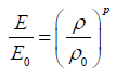
where E0 describes the nominal stiffness properties of the element. The task for the optimizer is to determine a density value for every element. The exponent p is a penalty parameter used to reach a result that is discrete as possible, by penalizing intermediate densities. If ρ tends to zero, the stiffness tends to zero too. This means, the element could be deleted because it is not important for the structure. If the density reaches a value of 1, the element is very important for the structure and may not be removed. This approach is called SIMP (Solid Isotropic Material with Penalization).
To illustrate the capabilities of the topology optimization, a simple example problem is illustrated here: Figure 1 shows the meshed design-space of a “truss”.


Here the entire space is considered design space. The task is to find a structure with a minimum volume and that the maximum displacement remains same as baseline. The baseline result is shown in Figure 2 with E = E0 = 210GPa, the maximum deflection at the node shown is 0.001826mm. After three iterations the density distribution or elasticity distribution as displayed in Figure 3 is arrived at. The “red elements” indicate a density = 1. This means these elements are very important and have their nominal stiffness properties. The “blue elements” have a density close to zero and therefore a very low stiffness and they can be removed. We can build the structure around the “red elements”.
The optimization problem in a finite element and multi-body dynamics software for the design, analysis, and optimization of linear structures can be stated as follows in equation (2)

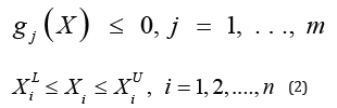
where f(X) is the objective function, g(X) are the constraints, both of which are functions of the design variables. There are m constraints and n design variables. The type of design variables can be size, shape/topography, and topology.
Topology optimization is a mathematical technique that generates an optimized shape and material distribution for a set of loads and constraints within a given design space. The design space can be defined using shell or solid elements, or both. The classical topology optimization can be set up solving the minimum compliance problem as well as the dual formulation with multiple constraints. Manufacturing constraints can be imposed using a minimum member size constraint, draw direction constraints, extrusion constraints, symmetry planes, pattern grouping, and pattern repetition
Post-World War II Wing Designs
Civil aircraft manufactured by Boeing, Airbus and McDonnell Douglas show that the layouts have been extremely stable in the post-World War-II era, with no dramatic variation between manufacturers, and between models of the same manufacturer, see Rao [2]. Wings made by these companies are based on the same few-spars-many-ribs design, with near-constant rib spacing, as may be seen in Figure 4 & 5. While most of the designs contain only two spars, a few include an additional mid-spar that goes partway, from fuselage up to wing-mounted engine.


An interesting variation is observed among some German aircraft dating back to the pre-World War II days. The old Heinkel bomber and the current Dornier aircraft both utilize iso-truss construction in the wing as shown in Figure 6

Here, we illustrate the topology optimization of an aircraft wing beginning with a fully solid wing to understand how this method allocates the material distribution with suggestions for removal and how such a structure resembles the design practices in place since World War II.
Topology Optimization of Solid Wing
A Solid wing made of Aluminum with Wingspan 13.5m, Constant chord wingspan 4.74m, Tapered chord wingspan 8.76m shown in Figure 7 is taken. The Chord length at wing root is 2.68m and at wing tip 1.39m. Material properties are taken as Young’s Modulus = 70000 MPa, Poisson’s ratio = 0.33 and Density = 2.60×10-09tonne/mm3.


The loads taken on the wing include flight load, fuel load and engine load. The airfoil sections, where pressure values are determined by Vortex Lattice method using XFOIL (a public domain code) are given in Figure 8. The pressure values at stations every 500mm apart the wingspan is given in Figure 9.
Fuel tank starts from 20% and ends at 85% of constant chord wingspan. Center of Gravity of the fuel tank is at 1.27m from leading edge and 2.5m from wing root. Fuel load is 1730 Kg per wing and is distributed through RBE3 element. The engine is mounted from 85% to 98% of constant chord wing span; its weight is 800 Kg. It is assumed to be mounted on front and rear spars through two ribs and the weight distribution at the four nodes of intersection between the two spars and ribs.
The wing was constrained in degrees of freedom analogous to a cantilever beam. Opti Struct optimization is adapted here. A linear static analysis was performed first, and the results were checked prior to setting up an optimization problem. It may be noted here that the baseline is a solid wing which will be heavy and rigid, and the results obtained here are of no consequence and hence not presented here. The next step is to setup an optimization problem on the finite element model. Material density of each element is a design variable which is defined using DTPL (Design Variables for Topology) card. In the present case, two responses from analysis (compliance and volume fraction) are defined using DRESP1 in which volume fraction (fraction of volume to be removed) is defined as constraint and compliance (inverse of stiffness) is defined as the objective function.


The classical setup involves subjecting the model to the objective of minimizing the compliance with volume fraction as constraint. Figure 10 shows material density plot obtained from the run along with what nature provides for such structures. Figure 11 shows iso-density boundary plot for the elements above density 0.2. Figure 12 shows how the objective function changed with respect to the iterations (41 in this case) until convergence is achieved.
It can be observed from Figure 11 that the resulting structure already resembles somewhat a classical wing type construction that can be adopted in the concept. We also observe from bird wings, how nature has designed them as feathery structures to reduce weight and provide minimum effort for propulsion. Optimization process leads to similar designs that nature provides. Here we have not constrained airfoil skin shape and a non-design space criterion is adopted in the next design case.
Next one layer of boundary elements was taken out of the design space to represent skin, see Figure 13. Extrusion manufacturing constraint was added to derive the location of spars. Extrusion constraint is used when it is desirable to produce a design characterized by a constant cross-section along a given path. Figure 14 shows iso-density boundary plot for the elements above density 0.3.


We can observe from Figure 14 that a single spar formation is suggested by the optimization process. To see whether a conventional 2 spar configuration is realized, another case is considered by splitting the wing into three regions. The result was a two-spar configuration, shown in Figure 15.
From these, we see that a conventional two spar configuration of a wing with several ribs as conceptualized from intuition and design practices followed right from the beginning of aircraft wing design since World War II is derivable through optimization. This gives us confidence of utilizing this powerful optimization technique for weight reduction of the existing designs or a minimum weight design that can be achieved for new designs.
With the information gathered so far, a new geometry with spars, ribs, stringers, hinge locations and lug attachments as shown in Figure 16 was considered. The objective was to derive material layout for ribs, hinge locations, stringers and cross section for front and rear spars, without flaps and ailerons. It has two spars viz. the front spar and the rear spar. There are two fuel tanks, one at the end of constant chord wings pan and the other in tapered chord wing span. There are three closely spaced ribs at the end of constant chord span for mounting the engine. It has six hinge locations attached to the rear spar and four lug attachments for mounting the wing to the fuselage bulkhead.


The given load on the wing includes flight load, fuel load, engine load and hinge loads (flap and aileron loads). Aircraft cruise condition was obtained for the flight load using Vortex Lattice method. Pressure distribution on the pressure surface is shown in Figure 17. The Plan-form of the wing was divided in to 200 panels and the pressure distribution was constant within each panel giving a discrete distribution. Plan-form from rear spar to the leading edge was divided in to seven panels. The discrete distribution of pressure on each panel from rear spar to leading edge is shown in Figure 18 and the division of panels in Plan-form is shown in Figure 19.


There are two fuel tanks. The capacity of the fuel tank is 2500 liters. The fuel tank at constant chord span takes 1000 liters and the fuel tank at tapered wing takes 1500 liters. The load was calculated using kerosene properties and distributed using RBE3 element see Figure 20.


Engine (800Kg) is assumed to be mounted on both front and rear spar along with three closely placed ribs at the end of constant chord wing span. Front spar takes 500Kg and the rear spar takes 300Kg. The load is distributed as shown in the Table 1. The weight distribution at the six nodes of intersection between the two spars and ribs is shown in Figure 21 as given in Table 1.

Since only one wing was taken into analysis (due to symmetry), symmetric boundary conditions were applied on the face nodes of front and rear spars. All the four lugs were constrained in all degrees of freedom. The boundary conditions applied are as shown in Figure 22.

Here the objective is to minimize compliance with volume fraction as constraint. Extrusion manufacturing constraints were added to obtain cross section for front, rear spars and stringers. Minimum member size control was added to all the design variables to penalize the formation of small members to obtain a discrete material distribution. Material density plot obtained for front and rear spars are shown in Figure 23. Elements which are having density above 0.3 are shown as Iso-density plot in Figure 24. Figure 23 & 24 suggest a box section for front spar and channel section for rear spar.


The iso-density plot for hinges of IB flap, OB flap and aileron are as shown in Figure 25 and suggests predominantly V-shaped members for hinges, as usually practiced. Material density and iso-density plots for ribs are shown in Figure 26 & 27. Figure 26 & 27 suggest a truss pattern for the ribs, once again a general practice adopted in the design of ribs. The regions in red are nondesign space. Finally, the iso-density plot for stringers is shown in Figure 28. This Iso-density plot suggests L-shaped cross section for stringers around the rear spar. Two stringers at the leading edge which are of not much significance in providing stiffness to the model are removed


The Final CAD Model without Skin and Stingers obtained from Opti Struct is shown in Figure 29. Eocyclotosaurus appetolatus that lived 240 million years ago before the first dinosaurs were provided by nature with animal load bearing structures is also shown in this figure. This is what was achieved in an aircraft structure (wing in this case) design in a long time consuming (4 to 5 years) using approximate engineering procedure including that of steps in testing. Today actual design takes one or two weeks using SBES as illustrated.

We can reduce the weight further by making a Composite structure of the wing as shown in Figure 30. Here optimized thickness for one of the ribs is only shown with CFRP. Total ply thickness in the ribs varied from 2.54 to 13.97mm; Similarly, for Spars and Skin. The mass saving obtained from the optimized CAD model Figure 29 to composite model in Figure 30 in the wing is around 35.7%.

Composite Rotating Blade Optimization
We now illustrate the process of designing a composite rotating fan blade (could be a propeller for a turbo-prop engine) from a given isotropic structure, see Rao [3]. The equivalent shell model of the fan blade is shown in Figure 31. The blades are of titanium, with E = 105GPa, μ = 0.23, ρ = 4.429×10⁻⁹kgm-3 and the hub is of stainless steel (non-design part). There are 18 blades and total mass excluding the hub is 3.722Kg. The 200mm long 65mm constant chord and 84o pre-twist blade rotates at 15000rpm.
As the blades are symmetric, only single blade (Mass = 206.8 grams) is used for composite optimization. The gas loads are neglected. The baseline stress field obtained is also shown in Figure 31. The peak stress is 343MPa.

Free vibration analysis of the metallic blade shows the fundamental mode to be at 107Hz. While obtaining a composite blade vane it should be kept in mind that the natural frequency at operating speed is sufficiently away from the critical speed on the Campbell diagram. With reduction in mass and increase in stiffness the natural frequency increases and here for the purpose of illustration of the process the frequency is minimized. Because of employing the composites, the stress level can be more than that allowed in metallic structure; however, for the purpose of illustration the peak stress is also limited to the baseline. The optimization process consists of three phases as outlined below.
Phase 1: Free size topology optimization
In this phase design concepts utilizing all the potentials of a composite structure are generated. By varying the thickness of each ply with a fiber orientation for every element, the total laminate thickness can change continuously throughout the structure, and at the same time, the optimal composition of the laminate at every point (element) is achieved simultaneously. Manufacturing constraints like lower and upper bound thickness on the laminate, individual orientations and thickness balance between two given orientations are also defined in this stage. Carbon Fiber is chosen whose unidirectional lamina properties are:
Volume fiber fraction = 0.5 Young’s modulus (in fiber direction) E11 = 115GPa Young’s modulus (perpendicular to fiber direction) E22 & E33 = 15GPa Shear modulus G = 4.3GPa
Variables: The Free size variables are taken to vary from 1.75 to 5.75mm from the blade ends (stacks 1 and 5) to the center varying along the blade profile length.

The design space is limited to the blade airfoil shape. The baseline is made of five patches (collectors) as in Figure 32 and the base laminate chosen is symmetric without a core with 0.4375mm thickness for all plies as given in Table 2. The inner stacks 2 and 4 have a total thickness 5.75mm with each individual ply 1.4375 mm thick. The middle stack 3 is 4.25mm thick with the individual plies 1.0625mm thick.


I bending natural frequency of the baseline composite blade is 109 Hz. The principal strains contour is given in Figure 33 with the maximum value equal to 0.002855.
There are 20 Ply Bundles in all, 4 each of 0o, +45o, -45o and 90o for the 5 Ply Orientations. Free Size Optimization gives the patch locations for each Ply Bundle. The results of all these plies are not shown here. The super plies obtained for each orientation are given in Figure 34. We notice that in all the cases of the super plies, the middle stack has maximum thickness of 1.438mm. The leading and trailing edges have minimum thickness.

Free Size Optimization resulted in the composite getting sized with plies dropping off from stacks 1 to 5. The number of plies in each stack after the Free Size Optimization is 13, 16, 16, 4 and 4 respectively.
Phase 2: Size optimization
Sizing optimization is performed to control the thickness of each ply bundle, while considering all design responses and optional manufacturing constraints.
The size optimization of the Plies obtained in Phase 1 with Free Size or Topology optimization is next performed to determine the thickness and laminate family within all the shell sections chosen in the blade. Objective functions are again mass and first mode and minimization of the same.
Two manufacturing constraints were incorporated:
a) Ply percentage for the 0’s and 90’s such that no less than 10% and no more than 60% exist.
b) A balance constraint that ensures an equal thickness distribution for the +45’s and -45’s.

The optimization results for total thickness are given in Figure 35 for all plies; with maximum thicknesses in the middle patch at the root given by 1.509, 1.344, 1.344 and 1.474mm respectively. The optimized blade natural frequency is 111 Hz slightly more than the metallic blade. Maximum principal strain given in Figure 36 is 0.003641 more than the baseline composite 0.002855. The weight saving obtained over the baseline metallic blades is 27%.

These ply bundles represent the Optimal Ply Shapes (Coverage Zones). The next step is to establish optimal stacking sequence including any manufacturing constraints. Ply thicknesses are directly selected as design variables. Composite plies are shuffled to determine the optimal stacking sequence with any constraints.
Phase 3: Ply stack optimization
A detailed design for Ply Stacking Sequence Optimization can be adopted by using Hyper Shuffle. Certain ply book rules are specified to guide the stacking sequence, e.g.,
a) Symmetric Stack Required
b) Number of plies in any one direction placed sequentially in the stack is limited
c) Stack is balanced, i.e. the number of 45o and -45o plies is the same.
d) Outer plies for the laminate should contain a particular ply (i.e. ±45o)
e) Minimize the number of occurrences of the 0° to 90° (or 90° to 0°) change in any two adjacent plies.
f) Minimize the number of occurrences of 45° to -45° (or -45° to 45°) change inside the stack by putting one 0° or 90° ply between them.
The stacking sequences obtained after four iterations of shuffling optimization are given in Table 3-7 for the five stacks used. Maximum film thickness in each of the stacks are as denoted in Table 3-7 and given below.


Stack 1: Maximum thickness is 0.414 + 0.00107 + 0.00682 + 0.011 + 0.407 + 0.00105 + 0.00746 + 0.011 + 0.407 + 0.00105 + 0.00746 + 0.011 + 0.414 = 1.669mm
Stack 2: Maximum thickness is 0.978 + 0.013 + 0.059 + 0.033 + 0.936 + 0.012 + 0.066 + 0.027 + 0.936 + 0.012 + 0.066 + 0.027 + 0.89 + 0.07 + 0.014 + 0.036 = 4.175mm
Stack 3: Maximum thickness is 1.262 + 0.095 + 0.137 + 0.013 + 1.097 + 0.084 + 0.144 + 0.017 + 1.097 + 0.084 + 0.144 + 0.0172 + 0.925 + 0.246 + 0.092 + 0.21= 5.664mm
Stack 4: Maximum thickness is 0. 986 + 0.931 +0.931 + 0.974 = 3.822mm
Stack 5: Maximum thickness is 0.4164 + 0.4085 + 0.4085 + 0.4164 = 1.649mm
A periodic oscillation is observed in the galloping of transmission wires in the northern states of Canada as shown in Figure 36. At subzero temperatures, when sleet is formed on the cables between the transmission towers located 100 m apart, they vibrate violently with more than a meter of amplitude under transverse wind conditions. Van der Pol in 1926 gave the concept of negative damping arising out of the sleet formation resulting in an airfoil like cable and showed that the large vibrations are due to instability (self-excited oscillations – relaxed oscillation), see the right-hand Figure 37. You may refer to Rao [4].

Another example of aerodynamic instability is observed on the Tacoma Narrows Bridge (called Galloping Gertie), in Washington State with its 1.9km span of the-then largest suspended bridge. It opened to traffic on July 1, 1940 and on windy days, motorists driving on it felt like being on a huge wave and would see the cars ahead disappear. On November 7, 1940, (four months after its opening) very strong winds sent the bridge into its rolling and undulating behavior a last time before collapsing, see Figure 38.

SBES and capability of simulating multi-physics in time domain had considerable influence on changing the approximate engineering and testing in evolving of new technologies in Aerospace Engineering, particularly in flutter. In almost all subbranches of Aeronautics, an excellent technological progress has been observed over the last two decades; Stability being more of significance in design of any aircraft. Multi-disciplinary optimization is being preferred over optimization for individual disciplines. When a fluid interacts with a solid structure, the flow exerts a pressure on the solid surface which may cause deformation in the structure. As a result, the deformed structure changes the flow field. The altered flowing fluid exerts another form of pressure on the structure. The repetition of the process occurs continuously. This is termed as Fluid-Structure Interaction (FSI). The study of the effect of aerodynamic forces on elastic bodies is termed as Aero-elasticity.
Flutter is most commonly seen on wings and the control surfaces of an aircraft structure. It is because of the load acting on these are the highest when an aircraft is in flight. The inertia and flexibility of the structure plays a very significant role in the aeroelastic dynamic stability of the aircraft. Self-excited and unstable oscillations due to unsteady aerodynamic forces from the air flow normally take place when a structural system which is under flow conditions beyond some threshold or critical value of the flow parameter like the dynamic pressure. Flutter can be basically a phenomenon of unstable oscillations in a flexible structure.

The 2D Flutter analysis of NACA 641 A212 done previously with a two way coupled FSI model is illustrated in Figure 39 with the structural and fluid domains, modal analysis results and pressure distribution over the wing surface. The vertical displacement obtained as a function of time for three velocities 100, 175 and 300 m/s loading conditions is given in Figure 40. The flutter case can be seen here.


For a three-dimensional analysis the wing derived in Figure 29 is adopted. Figure 41 & 42 give the details.
Figure 43 shows the mesh generated for the CFD analysis. The total number of nodes generated is 104742 and the number of elements is 357048. More care was taken towards refinement of the mesh to capture the flow physics exactly and to avoid negative volume error occurring due to the dynamic mesh in the analysis. The element quality parameters are: Skewness: ~0.95 and Orthogonality: ~0.02.


In the analysis, Mach number is taken as 0.8 for three angles of attack, 0.05, 5 and 25 degrees. The first four mode shapes are given in Figure 44. The fundamental corresponding to flapping is the first mode: 3.67 Hz; its natural time-period ~0.27sec. Considering 2 cycles, we have (0.27×2) = ~0.5 sec and thus the flutter duration considered for the analysis is 0.5s.
The fluid structure interaction in three dimensions under transient conditions is carried out with three different cases of angle attack viz., Case 1: 0.050. Case 2: 50 and Case 3: 250. The transient responses obtained are discussed here.
Case 1: Angle of attack 0.050
The dynamic FSI analysis for 0.5s at 0.050 with a time step of 0.001s at the tip is given in Figure 45 at 0.5s. Similarly, the fluid pressure at the wing tip is given in Figure 46.


Transient response at the wing tip is given in Figure 47. This clearly shows that the response is decaying without causing any flutter conditions. Figure 48 shows the frequency response of the time domain signal. Only one peak is present corresponding to I mode 3.67Hz.

Case 2: Angle of attack 50
The analysis was carried out for 0.81s at 50 with a time step of 0.001s. The results obtained are given in Figure 49 for the fluid pressure at the wing tip at 0.81s. Similarly, the fluid velocity at the wing tip is given in Figure 50.


In Figure 51 Pressure applied on wing exerted by the fluid is compared at the initial and final time steps as the peak pressure rose to the nose region. Figure 52 shows the wing displacement at the first- and last-time steps showing prevailing flutter conditions.
The flow streamlines at the initial time step indicate steady conditions, whereas at the last time step, the streamlines are not steady as shown in Figure 53. The response of the wing tip up to 0.81s is given in Figure 54 showing the flutter condition.


The above time domain analysis can be utilized for the crisis problem of 737 Max in Lion Air 310 failed flight on 28th October 2018 and Ethiopian Airline failed flight 302 on March 11th, 2019. Figure 55 shows the fluctuations in the vertical speed as against the expected altitude. The MCAS (Maneuvering Characteristics Augmentation System), shown in Figure 56 designed from going to stall did not function.
Figure 57 shows a lift coefficient CL as a function of angle of attack (AoA) α for a fixed wing.


where L is the lift force, S is the relevant surface area and q is the fluid dynamic pressure, ρ is the fluid density and u are the flow speed. Stall occurs at the maximum lift as shown in Figure 55 when AoA is further increased.
This condition of stall occurs when the aircraft nose points upwards at too greater angle, decreasing the aerodynamic lift. If the MCAS system is not designed carefully, it can force the aircraft nose down. Today’s technology with multi-physics as discussed in the previous section allows a time domain analysis taking into the relevant existing parameters like temperature, pressure … to prevent or correct the instantaneous AoA to keep the plane safely during take-off period.
Closure
The aircraft structures are the first ones that adopted modern designs of weight reduction of aircraft structures using the concept of topology optimization and composites. The same followed with rotating structures of fan blades and propellers, flutter design of aircraft structures like wings. Multi-Physics developed during Science Revolution period bounced back with the advent of High- Performance Computing. Recent stall issues of failures are also discussed that could be addressed by time domain analysis and multi-physics.
The author is very thankful to his students and colleagues for having contributed to these works. The author is also grateful to his wife Indira Rao for her support throughout his career.
References
- Rao JS (2011) History of Rotating Machinery Dynamics. Springer.
- Rao JS, Kiran S, Chandra S, Kamesh JV, Madhusudan AP, et al. (2009) Topology Optimization of Aircraft Wing. Journal of Aerospace Sciences & Technologies 61(3).
- Rao JS (2013) Optimization of Fan Blades. The Ninth International Conference on Vibration Engineering and Technology of Machinery, VETOMAC-IX, 21-23 August, Nanjing, China.
- Rao JS (2019) Vibrations through SBES, Krishtel publication, Chennai, India.


