


Toward a Noninvasive Measurement Method of CO2 Arterial Pressure
Aicha Rima Cheniti1*, Hatem Besbes2, Moez Chafra3, Christophe Sintes4 and Mohamed Omri5
1Laboratoire de recherche structure et mécanique appliquée, Ecole polytechnique de Tunis, Université de Carthage, Tunisia
2Faculty of Sciences, Department of Physics, King Abdulaziz University Jeddah, Saudi Arabia
3Laboratoire de recherche structure et mécanique appliquée, Ecole polytechnique de Tunis, Université de Carthage, Tunisia
4Lab-STICC, ITI Department, Telecom Bretagne, Technopole Brest-Iroise, France
5Deanship of Scientific Research, King Abdulaziz University Jeddah, Saudi Arabia
Submission: October 06, 2020; Published:October 28, 2020
*Corresponding author:Aicha Rima Cheniti, Laboratoire de recherche structure et mécanique appliquée, Ecole polytechnique de Tunis, Université de Carthage, Tunisia
How to cite this article:Aicha Rima C, Hatem B, Moez C, Christophe S, Mohamed O. Toward a Noninvasive Measurement Method of CO2 Arterial Pressure. Curr Trends Biomedical Eng & Biosci. 2020; 19(5): 556025. DOI:10.19080/CTBEB.2020.19.556025
Abstract
Until now, the measurement of carbon dioxide blood pressure is done ex-vivo, using an invasive process. This paper describes a first step toward a novel noninvasive process for in-vivo measurement of this pressure. As first approximation, the blood solution is modeled as a simple aqueous solution of carbon dioxide in a cylindrical rigid canalization. The Drift flux model and the Young-Laplace equation are employed to describe the fluid behavior. The numerical model relates the carbon dioxide pressure through the mixture pressure and velocity. The spatial distributions of these parameters are implemented to create linear mathematical relations between the mean mixture pressure and the radial velocity variation. As long as we are interested in a non-invasive measuring of the carbon dioxide pressure, a response model is proposed to describe the ultrasound signal backscattered by the considered solution. The linear relations are applied to deduce the carbon dioxide pressure through the measured radial velocity difference, using two computing methods of ultrasound signal. A comparative study is made between them showing the more appropriate process to compute the carbon dioxide pressure.
Keywords: Drift Flux Model; Carbon Dioxide Pressure; Mixture Pressure; Radial Velocity; Ultrasound
Introduction
Artificial ventilation is a medical practice used in pneumology services, operating rooms, ICU intensive care units, etc. It is a method for compensating insufficient breathing or replacing a breathing inefficiency or lack of ventilation in intensive care units. Several parameters are needed to control the patient artificial ventilation such as blood pH, arterial oxygen pressure and arterial carbon dioxide pressure [1,2]. Arterial blood gas (ABG) analysis is a medical procedure used to measure these three settings. The ABG aims to diagnose and monitor gas exchange of patients with respiratory failure including those undergoing mechanical ventilation. The analysis is invasively done by sampling blood from the radial artery located at the wrist, using a needle and a syringe. The sampling is analyzed in laboratory with an analytical instrument. Actually, ABG is the only method existing to measure partial pressures and arterial pH [3,4]. This method is a subject of some problems. The patient is likely to have contaminations, infections or necrosis due to a local blockage or decrease of blood flow. The sampling presents also accident risks by using the needle stick. It can as well create inflammations around the site of puncture. Except the pain that the patient feels during the procedure, the sampling cannot be executed daily. In fact, this can cause anemia, due to the excessive amount of collected arterial blood [5].
These problems mainly provided insights into a noninvasive procedure for carbon dioxide pressure measurement; a new method making a continuous control to obtain frequent and real-time results via ultrasound. It is the first time that a numerical model is used to develop a system for measuring arterial carbon dioxide pressure. As a first approximation, the arterial blood solution was modeled as a two-phase flow moving across a constricted rigid cylindrical tube with a constant cross-section. The mixture is composed of two phases: a gas phase which was carbon dioxide and a liquid phase which was an aqueous carbon dioxide solution. The behavior of the considered two-phase flow mixture was mainly described by the Young-Laplace equation and the Drift flux model which is governed by physical laws of energy, momentum and mass. Findlay and Zuber were the first founders of the Drift flux model [6] and the concept was detailed by Yang et al. [7], Ishii [8]and Shang [9]. The Drift flux model relates mixture velocity and pressure [8] while the Young-Laplace equation relates the two-phase pressures [10]. Mathematical relations were created through the simulation results of the mixture velocities, the carbon dioxide pressure and the mixture pressure. They were implemented to compute the mean mixture pressure through the radial velocity variation. In a second step, the considered fluid’s response via ultrasound was modeled through its mechanical parameters. Two measurement methods using ultrasounds for the determination of the mean carbon dioxide pressure were simulated in correlation with the created mathematical relations.
ABG Technique
Arterial blood gas (ABG) sampling presents a measurement system meant for obtaining information about the respiratory status of the patient (arterial oxygen and carbon dioxide pressures), and the acid-base balance. The radial arterial blood sampling process consists of:
a. Palpating the radial artery with index finger around the planned puncture site
b. Holding the ABG syringe and inserting the needle through the patient’s skin at an angle of 45° over the point of maximal radial artery pulsation (Figure 1),
c. Advancing the needle into the radial artery until observing blood flashback into the ABG syringe which will be filled under arterial pressure,
d. Obtaining at least 3 ml of arterial blood,
e. Withdrawing the needle when the required amount of blood has been collected and removing the needle from the syringe [3,4,11].

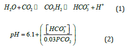
The syringe is placed in the ice, and immediately sent to the laboratory for analysis to ensure results accuracy. The samples should be analyzed as quickly as possible to avoid the effects of continued metabolism, and to limit the loss of potassium by red blood cells and the diffusion of oxygen through the plastic syringe. The sample taken is inserted into an analytical instrument that uses electrodes to measure the pH of the plasma solution (Clark electrodes) and the partial pressures of the carbon dioxide (Severinghaus electrodes) and oxygen (Sanz electrodes) [3,4,13]. The Severinghaus electrode is a glass electrode set in a bicarbonate solution which is contained in a nylon spacer and separated by a membrane from the sample. The carbon dioxide diffuses out of the blood sample through the silicone membrane and into the bicarbonate solution, altering the initial pH (reaction (1)). The hydrogen H+ are measured by a modified pH cell. The hydrogen ions’ number generated within the bicarbonate solution is proportional to the pressure of the carbon dioxide PCO2 (equation 2) [3,14].
Theoretical Method
Mathematical modeling
Arterial blood is a complex, heterogeneous and non-Newtonian fluid, since it contains various cells and substances suspended in plasma solution. Carbon dioxide CO2 and oxygen O2 are gases which are transported into two forms in blood: gaseous form and dissolved form. The gaseous form is responsible for creating the arterial gas pressures causing the dissolution of a fraction of each gas [11,15]. In view of the fact that we are intent to estimate the carbon dioxide pressure in arterial blood PaCO2, the plasma and the considered gas are supposed to be isolated and considered as a two-phase fluid. The fluid consists of an aqueous solution of carbon dioxide (liquid phase or continuous phase representing the plasma solution) and the carbon dioxide gas (gas phase or dis persed phase). The mixture was considered as a Newtonian incompressible fluid, moving horizontally across a constricted rectilinear rigid tube with a constant cross-section. Different models exist to describe the two-phase flow. The most considered models are the homogeneous equilibrium mixture model HEM, the two-fluid model and the Drift flux model [16-18].
Homogeneous equilibrium mixture model
The homogeneous equilibrium mixture HEM is used to conceive a homogeneous two phase flow. The phases are supposed to be well mixed, strongly coupled and move at the same velocity with the same temperature. The model is described only by one set conservation equations governing the balance of energy, momentum, and mass [16]. The HEM is used to study many cases like water-steam mixtures, cardiovascular and respiratory system, blood flow, etc. [18,19]. The HEM cannot be adopted to model our fluid because the three mentioned equations do not express the gas phase.
Two-fluid model
The two-fluid model considers each phase separately bounded by moving interfaces; the two phases are weakly coupled. The model is described by three conservation equations governing the balance of mass, momentum, and energy of each phase [17,20]. The two-fluid model is applied in many important domains for example in the case of oil and refrigerant mixture in boiling water, compressors and accumulators, pressurized water nuclear reactors, chemical reactors and two-phase flow lubrication [18,21]. The two-fluid model does not match with our request because it does not consider a relation permitting to determine gas parameters through the liquid velocity.
Drift flux model
The Drift-flux model treats the two separate phases as coupled in one phase. The mixture properties make the Drift-flux formulation simpler than the two-fluid model formulation. This model considers the mixture as dynamic where the two phases’ components are coupled. The velocity of the two fluids is assumed to be monitored by a mean velocity of the mixture completed with a constitutive relation for estimating the relative motion between the two phases (called drift velocity) [6,8,18].
To apply this model, we assume:
a. The mixture flow is steady, in the two dimensions (z, r).
b. The two phases are incompressible.
c. The flow is axisymmetric.
d. The velocity component Vzm depends only on the flow direction (z-axis)
The governing equations are:
i. Mixture Continuity Equation
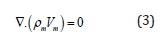
ii. Continuity Equation for Dispersed Phase
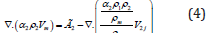
iii. Mixture Momentum Equation

where
ρm: mixture density
Vm: mixture velocity vector
α2: volumetric fraction of gas
ρ2: gas density
ρ1: liquid density
Г2: generation rate of gas phase
pm: mixture pressure
μm: mixture viscosity
gm: gravitational acceleration vector
V2j: drift velocity vector of the gas phase with respect to the volume center of the mixture
Mm: interfacial force
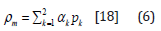
The mixture density is given by:
The axiom of continuity is conditioned by
The mixture pressure is expressed by:
The drift velocity is determined by the following relation:
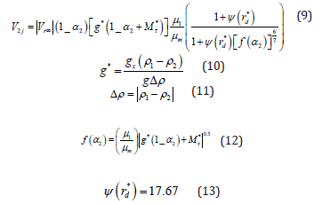
Where:
αk: volumetric fraction of kth phase
pk: pressure of kth phase
Vr∞: terminal velocity
Mτ*: transverse stress gradient
gz: component of gravitational acceleration vector along the axis of flow
g: gravitational acceleration vector
The Drift flux model was chosen to describe the studied mixture flow. In fact, this mathematical model allows the correlation between flow velocity, mixture pressure, the relative velocity and the physical parameters of both phases. Therefore, the Drift flux model can be used in experimental applications, as it is able to determine the characteristics of both phases (like velocity, pressure, etc.) by measuring mixture velocity. Therefore, the drift-flux model allows establishment of a relationship between the mixture velocity and the mixture pressure. Thus, the measurement of velocity permits the detection of pressure value.
Young Laplace equation
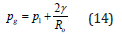
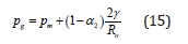
The gas phase took a micro-bubbles form suspended in the mixture. An interface exists between the two non-solid substances, where there is a pressure interaction described by the Young-Laplace equation [10,23]:
where
pg: gas pressure
pl: liquid pressure
R0: microbubble’s radius.
γ: surface tension
The Young-Laplace equation and the Drift flux model allow the determination of carbon dioxide pressure pg once the mixture pressure pm and mixture velocity Vm are known.
From equations (8) and (14), the carbon dioxide pressure is expressed by:
Evolution of the system according to the mean mixture pressure
The heart pressure essentially assures the arterial blood motion. Seen from this angle, the dominant velocity component of the fluid is certainly the axial one. Therefore, in ultrasound explorations, the axial velocity is measured by the Doppler mode. As already said, in arterial blood gas analysis, the blood is taken by a needle inserted at 45° for the skin. In this case, the blood is essentially propelled by the gas pressure into the syringe (essentially the blood radial motion) [3,4]. Thus, the radial velocity can be used to determine the mean mixture pressure and consequently the mean carbon dioxide pressure. The mathematical model presented in section 2 describes the mixture in general case. Changing initial conditions, the calculation provides new values of mixture parameters. The variation of radial velocity Vrm along z axis was studied according to the mean mixture pressure Pmoy. The latter was calculated by summing the pressure values in different cells of the measurement domain divided by the number of cells.
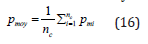
where
pmi: pressure in ith cell of the measurement domain
nc: number of cells in the measurement domain
The radial velocity behavior depends on several parameters such as initial conditions which must be fixed at the beginning of each simulation. Changing these conditions gives different results expressing the evolution behavior of velocities, pressures and the volumetric fraction of gas. For every simulation, the governing equations resolution gave a distribution of the radial velocity Vrm as a function of the mean mixture pressure Pmoy. Then, mean pressure levels occurred through radial velocity Vrm in different positions (z,r).
Computation of the mean mixture pressure and the mean gas pressure through radial velocity variation The mean mixture pressure levels were employed to identify a method for the computation of the mean mixture pressure by the measurement of the radial velocity. First, the initial pressure levels were exploited to reach new levels through the variation of radial velocity between two z positions. Secondly, the new pressure levels were interpolated by linear functions of r positions. Using these functions, it was possible to compute the mean mixture pressure Pmoy by the radial velocity gradient. The mean carbon dioxide pressure pgm is calculated by the following expression:
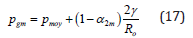
The mean volume fraction of carbon dioxide α2m is calculated by:
Where
α2i: the volumetric fraction of the carbon dioxide in the ith cell.
The α2m was considered as a constant parameter. This corresponds to the current measurement method that suppose the same conditions when measuring the arterial carbon dioxide pressure in a fixed volume.
The Ultrasound Waves as a Solution for the Measurement of Fluid Mixture Radial Velocity
Ultrasound is a technique employed in many fields like industry, medicine, research etc. Ultrasound system uses incident acoustic waves to intercept reflected signals and process them. In medicine, the received information is sometimes exploited to measure the blood flow velocity. It relies on the ultrasound trans mission to the blood vessel. The reflected ultrasound is picked up by the ultrasound probe. The reflection comes mainly from red blood cells. The velocity of the target can be estimated by measuring the frequency difference between the incident wave and the echoes intercepted after reflection on the target [24,25]. This difference is called the Doppler frequency; it is directly proportional to the flow velocity along the ultrasound beam. It is expressed by the following Doppler Law [24,25]:

Δf = Doppler shift
V = axial blood velocity
θ = angle between the vessel axis and the ultrasound beam
fe = ultrasound incident frequency
c = ultrasound velocity
Results
The resolution of the numerical model requires application of an algorithm treating the pressure-velocity coupling in the momentum conservation equation and the volumetric fraction-velocity coupling in the conservation equation. The governing equations of the Drift flux model was solved by the Mass Conservation Based Algorithm (MCBA) [26]. The resolution respects the following steps:
a. Guessing initial values of the mixture velocities and pressure as well as the volumetric fraction of carbon dioxide
b. Solving the momentum equation for the mixture velocities
c. Solving the pressure-correction equation founded by the mixture continuity equation
d. Correcting mixture velocities and mixture pressure
e. Solving the continuity equation for dispersed phase
f. Repeating the previous steps until the achievement of the results’ convergence
For the purpose of numerical computations, the physical parameters were setting. The choice of different values was inspired from the effective arterial reality in normal conditions (T=37°C). The liquid density ρ1 was equal to 996 kg/m3, the carbon dioxide density ρ2 was equal to 1.87 kg/m3, the liquid viscosity μ1 and the carbon dioxide viscosity μ2 were set respectively at 0.717 10-3 Pa/s and 15.2 10-6 Pa / s, the surface tension of water γ was 7.10-2 N/m [27-29] and the carbon dioxide bubble radius R0 was 10-6 m. The considered flow field had a cylindrical shape of a constant section with a radius of 4.10-3m (with reference to radial artery diameter) and a length of 10-1 m (with reference to the subsequent measurement possibilities). The computational domain was divided into finite volumes described by uniform grids with 10 cells in each direction (z,r). The samples of velocity components Vzm and Vrm were respectively 10x9 and 9x10 while the samples of the mixture pressure, the volumetric fraction and the pressure of carbon dioxide were 9x9 (Figure 2). The no-slip condition was adopted, the radial velocity Vrm was zero at the level of the pipe walls. The values of mixture pressure, volumetric fraction and velocities were maintained constant at the inlet and outlet of the two-phase mixture.

The numerical simulations were carried out in 2D based on the parameters values fixed above. By following the steps of the MCBA algorithm, the spatial distributions were assigned. The velocity Vzm increased at the inlet of the pipe and then became approximately constant before reaching the outlet boundary (Figure 3a). Then, it decreased to attribute the values set at the output. The Vrm (Figure 3b) underwent a clear variation near the pipe’s center. Moving away from the center, the velocity values became negative and decreased until reaching zero at the wall contact, according to the non-slip condition. The mixture pressure pm (Figure 3c) and carbon dioxide pressure pg (Figure 3d) had an increasing profile in the beginning and after they decreased along the z-axis until the exit of the considered tube. Along the r-axis, the pressures dropped from the center of the tube to the wall. The volumetric fraction increased from the tube center to the walls (Figure 3e). This can be explained by the tendency of the gas micro-bubbles to move towards the walls. The increase of α2, along the r axis, was due to the decrease of the mixture pressure. Simulation results shown in Figure 3 presented mixture behavior for one case of initial conditions. In order to study the effect of the mean mixture pressure on the radial velocity, the initial conditions were modified, and new simulations of pressure and velocity were made

The results of radial velocity variation along z axis, for different mean mixture pressure values, were used to deduce families of functions Pmoy= f (Vrm) for different (z,r) positions. Therefore, the determination of a given value of radial velocity for a known position (z,r) enabled mean mixture pressure calculation. The radial velocity variation was described as a function of the mean pressure along the z axis for different r positions. Thereby, these typical functions facilitated the creation of pressure levels as a function of radial velocity Vrm at a known position (z,r). The levels were limited to a specific position which are z = 3 and z = 8. Using these two sites, it was possible to compute the mean mixture pressure Pmoy by the radial velocity variation between z = 3 and z = 8, for positions r ranging from 2 to 9 (Figure 4a). It was convenient to choose well-defined positions to create a relationship between the considered pressure and the difference of radial velocity (Figure 4b). Thus, the first three positions were adopted to determine Pmoy. The results of positions r = 2 and r = 3 were expressed by a quadratic function as:
Position r=2:

Position r=3:

The functions calculated for the first two radial positions were exploited to measure the mean mixture pressure. The first equation (20) allowed to calculate Pmoy and the second one (21) was used to verify the measured pressure value.

Modeling of the System Response Using Ultrasound
The simulation results were exploited according to two positions of the flow axis. In fact, ultrasonic waves are transmitted to two linear rows along the radial axis for the positions z = 3 and z = 8 perpendicularly to the flow axis. Due to the scattering phenomenon, a part of the transmitted energy amount is reflected through different directions producing a useless information for our system (signal noise). Ultrasonic waves are estimated to be scattered once through the structure. The received signal contains only the useful information through the position, the velocity and the gas microbubbles number of the in signified sample of the measurement domain. The elementary signals as well as the total response of the two positions z = 3 and z = 8 were modeled by frequency and amplitude calculation.
Frequency
The transmitted ultrasound is scattered by carbon dioxide microbubbles moving in the mixture, the frequency of backscattered energy is different from the transmitted onef0. The difference between the frequency of the elementary signal fi and the transmitted frequency f0 is determined by the Doppler effect. This difference is calculated by [25,30]:

The radial velocity Vrm is calculated through the previous simulations. The ultrasound fixed velocity c is 1500m/s. The incident frequency f0 is 10Mhz (small depth).
Backscattered energy
The elementary signal amplitude depends on the ultrasound backscattered energy of the crossed structure. The first structure that interposes the waves propagation is the pipe wall of the mixture. The incident ultrasound waves interact with the wall, an energy’s amount is reflected due to the acoustic impedance changing of the propagation medium and detected by the receptive transducer. The remaining part undergoes a refraction and continues to propagate in the mixture (Figure 5a). The transmitted acoustic intensity It is given by the following relation [24,25]

where
I0: incident intensity
T: transmission coefficient of the amplitude
Z1: boundary impedance
Z2: mixture impedance
The transmitted part of energy continues to propagate through the fluid solution and undergoes attenuation phenomena. The transmitted intensity Iti at the output of the ith voxel is given by [24]

where
I0i: transmitted intensity at the input of the ith cell
Ri: traveled distance to the ith cell
α: attenuation coefficient
The acoustic intensity located at the ith cell’s input undergoes already interactions in the previous cells before arriving at the ith cell (Figure 5b).

Another phenomenon is created. In fact, the gas microbubble behaves as a point source scattering a part of the wave in all directions of space. The amount of backscattered energy depends on the microbubbles number and surface exposed to ultrasonic waves. The equivalent surface σs of a microbubble oscillating in a liquid medium is given by [30,31]:

Where
w0= natural microbubble’s frequency
w= frequency of transmitted ultrasound
ρl= liquid phase density
μl= liquid phase viscosity
C= sound velocity in the liquid
C1= coefficient of correction
The microbubble’s pulsation w0 is given by [31,32]:

Where
P0= ambient pressure
γ= surface tension coefficient.
κ= gas compressibility
The correction coefficient C1 is calculated by the wavelength of acoustic wave in the liquid phase λ and the radius of gas microbubble R0. It is given by [31,32]:

The backscattered intensity due to the scattering phenomenon in the ith cell is determined by the equivalent surface σs, the number of gas microbubbles nbi and the received intensity at the cell’s inputI0i. The microbubbles’ number nbi in ith cell of the measurement domain is estimated by the distribution of the volumetric fraction of the carbon dioxide. It is given by:

α2i = gas volumetric fraction in ith cell.
Vc= cell volume
Vb= gas microbubble volume
Then, the backscattered intensity caused by scattering phenomena Ibi is calculated as [32]

Taking into account all the cited phenomena, the received intensity at the ith cell’s input I0i is determined as

Thus, the backscattered intensity Iri is calculated by the intensity I0itaking into account only the absorption in return. It is given by the following expression:

The backscattered ultrasonic pressure is calculated by three parameters as follows [24]
Mixture response
The system was excited by two ultrasonic pulses which both duration is equal to τ (the duration is fixed according to the size of the sample to be studied), one pulse for the position x = 3 and another for the position x = 8. The backscattered ultrasound pressure of every cell takes a signal form. The elementary signal’s characteristics depend on the radial velocity of the ith sample, the microbubbles’ number and the arrival time. The response was modeled by a sinusoidal signal modulated by a Gaussian. Thus, the elementary signal of the ith cell was determined by the frequency fi and the acoustic pressure pri presenting the signal’s amplitude. The form of the signal si (t) is given by:
fi: signal frequency of ith cell
fg(t) is the Gaussian function, it is given by:
σ: the standard deviation
t: time
Each received answer is summed to the previous one taking into account the arrival time of the elementary signal. The total signal s(t) of each x position is calculated by:
nc: total number of cells
di: distance between the ith cell and the transducer
Determination of Mixture Parameters Through Mixture Signal Response
First calculation method A first method (method M1) is used to determine radial velocity difference and to deduce the two mean pressures. It consists on measuring the frequencies of the cells at the radial position r = 2 and r=3 for both z = 3 and z= 8, using the spectra. Then, radial velocity differences are calculated through these frequencies. The first ultrasound transmission was used to determine the response of positions r = 2, z=3 and r = 2, z=8. The rectangular windowing method was applied to the two total signals for extracting the considered responses. The frequencies were determined through spectra of the two signals by applying the Fourier Transform, allowing the radial velocities to be identified at the two linear positions for r = 2. A second transmission was made to determine the response of position r = 3, z=3 and r = 3, z=8. The same calculation procedure was adopted to estimate the radial velocities of the considered positions.
Second calculation method
A second method (method M2) is adopted to estimate the radial velocity differences between the positions z = 3 and z = 8 at r = 2 and r = 3. The method M2 calculates the difference between the two received signals and allow the radial velocity differences to be read directly from the frequency spectrum. This method was applied for the signals coming from the position (r = 2, z = 3) and (r = 2, z = 8) and the signals coming from the position (r = 3, z = 3) and (r = 3, z = 8). Then, the frequencies were calculated through signal differences spectra for the same theoretical Pmoy values adopted in method M1.
Results
The system response’s modeling via ultrasonic waves was based on different characteristics of the mixture which are the radial velocity Vrm, the volumetric fraction α2 and the position of the samples. The answer concerned the linear positions z = 3 and z = 8. For each row z, the signal was calculated at each radial position.
Under specific initial conditions, numerical simulation provided the different cells responses in the position z = 3 and the position z = 8. Two spectra are deduced from the total signals of position z = 3 and z= 8. Both spectra contain some peaks corresponding to the cells response (from r = 8 to r=2). The peak of every spectra corresponds to a dominant frequency compared to others (Figure 6). The method M1 was applied for various values of the pressure Pmoy altering between 2kPa and 40kPa, for the positions (r = 2, z = 3), (r = 2, z = 8), (r = 3, z = 3) and (r = 3, z = 8). For each received answer, theoretical frequencies and response frequencies were calculated. The radial velocity of each position was determined by the response frequency using relation (22). Subsequently, the difference of velocities ΔVrm between the two positions makes the possibility to calculate Pmoy by relations (20) and (21) in the considered positions.

The relative error of Pmoy measurement was calculated for the position r = 2 and r = 3 (Figure 7a). The blue curve describes the evolution of the relative error for r = 2. This parameter undergoes fluctuations between 0.02 and 1. First, the relative error decreases from 1 to 0.06 when the mean mixture pressure increases to 9kPa then from 0.4 to 0.02 with a rise from 20kPa to 30kPa. A small increase from 0.06 to 0.4 appears for a pressure varying between 9kPa and 20kPa. The second green curve describes the relative error variation for the radial position r = 3, between 0.02 and 0.5. The points of the two curves do not completely coincide, there is a coincidence in four points: 3rd, 4th, 7th and 8th simulations. It is remarkable that the position r = 3 gives mean pressure values closer to theoretical ones, since its relative error is less than the position r=2. Theoretical frequency differences and response frequency differences were calculated for the two positions r = 2 and r = 3 by the second method M2. The radial velocity difference of each z position is determined directly by the calculated frequency difference. Subsequently, the mean mixture pressure of the position r = 2 and the position r = 3 is also deduced by the two relations (20) and (21). The variation of the relative error for different values of Pmoy for the two positions are observed through (Figure 7b). The blue curve corresponding to the position r = 2 shows a decrease of the relative error when the mean pressure increases towards 20kPa then a small increase towards 40kPa. The second green curve corresponding to the position r = 3 presents a decrease of the relative error when the mean mixture pressure rises towards 10kPa. The relative error undergoes a small increase up to 0.2 between 10kPa and 15kPa then a decrease to 0.02 for 25kPa. This parameter stabilizes at 0.09 for 40kPa. The two curves do not coincide at any point. For the majority of simulations, the position r = 3 gives closer values of mean pressure as compared to those of the position r = 2 except for the fourth and fifth simulations whose relative errors are lower for the position r = 2 but they are close to the error values of the position r= 3.

Discussion
The strategic goal of this work was finding a novel noninvasive measurement process of the carbon dioxide arterial pressure. In first approximation, the blood was modeled by simple aqueous solution of carbon dioxide. The mechanical study of this solution was done by adopting the Drift flux model. It describes the motion between phases considering the mixture velocity and the relative velocity. The objective of this research is to establish a relationship between the pressure of carbon dioxide and the radial velocity of the considered solution, using the Young Laplace equation, the continuity equation for dispersed phase, the continuity equation of the mixture and finally the mixture momentum equation. The first three equations of Drift flux model were obviously chosen to determine the mixture pressure through the radial velocity which is influenced by the carbon dioxide pressure. The use of Young Laplace equation was substantial to calculate the pressure of carbon dioxide through the mixture pressure. Since the ultrasound detects the velocity of the hole mixture, it was convincing that the Drift flux model affords the possibility to define the gas pressure through the considered parameter.
It can be stated that the results of the model simulation reached to create levels of the mean mixture pressure, which were used to deduce a method for calculating through the radial velocity measurement by ultrasound. The latter parameter is influenced by the carbon dioxide pressure. Therefore, the levels were based on this parameter. In practice, it was not appropriate to make simultaneous measurements of the radial velocity in all the considered positions along the z and r axis. This required several ultrasonic transducers. The placement of these sensors near to each other created a confusion of information detected from each cell of the measurement domain and increased the signal noise which created measurement errors. To overcome these problems, it was necessary to restrict the number of sensors. The use of two ultrasonic transducers fixed perpendicularly to the flow direction can of course fulfill more precision than one. The two positions must be relatively distant to minimize errors in measuring the radial velocity. The choice was oriented to the axial positions z = 3 and z = 8 because there was a significant variation of velocity between these two positions and to avoid boundary effects. Thus, both sensors were able to measure the mixture radial velocity in the field of view.
The findings through this two positions are particularly important in the sense that they facilitate the computation of the mean mixture pressure knowing the radial velocity difference. The second and the third locations along the radial axis were employed because of the linear behavior of the function Pmoy=f (ΔVrm). Equations (17), (20) and (21) are the first main results of the current study. They allow the calculation of the mean mixture pressure and the mean gas pressure. In addition, the linear equa tions present a massive advance because they constitute a very simple and reliable method compared to the actual arterial blood gas sampling. It is remarkable that ABG technique makes measurement uncertainties because of its multiple steps from blood extraction until pH measurement of a plasmatic sample. Thus, there will be certainly difference between equilibrium in vivo and equilibrium ex vivo due to difference steps of sample extraction and processing (for example the amount of gas that can be found in the syringe at measurement date). The ultrasound process can be done with conservation of all properties of the blood solution, this because it works without opening the blood system and then without any alterations of the latter equilibrium.
The second main results of this study are the ultrasound method employed to read the radial velocity variation ΔVrm. At the location r=2, the relative error determined by the method M2 is lower than the first one for a mean pressure value around 5kPa and for values varying between 10kPa and 25kPa.Elsewhere, the method M1 provides lower values than M2. Generally, the method M2 is more stable than the methodM1that shows significant fluctuations compared to M2 (Figure 8a). For the location r = 3, the relative error of the first method M1 is lower for a mean pressure reaching 5 kPa otherwise it becomes larger than the second method M2 (Figure 8b). The weighted arithmetic mean of the relative error is calculated, giving a value of 0.13 for the first method M1 and 0.11 for the method M2. Concerning the position r = 2, the weighted arithmetic mean of the relative error is equal to 0.23 for the method M1 and equal to 0.31 for the method M2. Thus, it can be stated that the two methods give close results to the mean mixture pressure’s values calculated for the radial locations r=2 and r = 3. This parameter is then used to determine the carbon dioxide pressure, assuming at this stage that the mean volumetric fraction of the gas is approximately constant. The implementation of this system is possible and easy since it does not require specific skills or knowledge in anatomy or medicine in general. The radial artery can be brought out by a classical method using a garrote and the two transducers are settled down in the chosen positions. The experimental studies will be setup to improve and validate theoretical results.
Conclusion
This work constitutes a first step in the pathway toward performing a novel system for noninvasive in vivo measuring the arterial blood pressure of carbon dioxide. For this, a first numerical model had been adopted and as first approximation, the blood solution was modeled by an aqueous solution of carbon dioxide in a rigid cylindrical canalization. The calculation of the carbon dioxide pressure was done following a drift flux model combined with Young-Laplace equation. This allowed the establishment of a relationship between the carbon dioxide pressure and the radial velocity variation (ΔVrm) at different position (r,z). As long as it’s about measuring a fluid velocity, two numerical simulation methods using ultrasound waves, interacting with carbon dioxide microbubbles, were proposed. The first method M1 determines the radial velocities of the cells at the radial positions r = 2 and r=3 for both locations z = 3 and z= 8, through the spectra. Then, the velocity differences are calculated for r = 2 and r=3. The second method M2 measures the frequency differences between the considered positions, then the radial velocity variations are computed by the Doppler effect. The linear relationships, established through the numerical model, were employed to deduce the mean pressures of the mixture and carbon dioxide from the radial velocity variation. The calculation of incertitude for the two methods showed differences in performances depending on the pressure values. This can be subsequently verified when experimental measurement will be done. If the future measurement coincides perfectly with calculated results, this can offer different measurement regimes with the same system.
References
- Ashfaq H (2010)Understanding mechanical ventilation. A Practical Handbook Second Edition. Springer, London, UK.
- John BW(2012)Respiratory Physiology, The essentials. Ninth Edition. Lippincott Williams & Wilkins, a Wolters Kluwer business, China.
- Ashfaq H (2009) Handbook of Blood Gas/Acid-Base Interpretation. Springer, London, UK.
- Iain AMH, Alan GJ (2007)Arterial Blood Gases made easy. Elsevier, China.
- Radiometer (2011) Le guide du gaz du sang. Radiometer Medical Aps, Denmark.
- Zuber N, Findlay JA(1965) Average volumetric concentration in two-phase flow systems. J. Heat Transfer 87(4): 453-468.
- YangRC, Zheng RC, WangYW(1999)The analysis of two-dimensional two-phase flow in horizontal heated tube bundles using drift flux model. Heat and Mass Transfer 35: 81-88.
- Ishii M(1977)One-dimensional drift-flux model and constitutive equations for relative motion between phases in various two-phase flow regimes. Technical Report ANL-77-47, Argonne National Lab Report, USA.
- Shang Z (2005) CFD of turbulent transport of particles behind a backward-facing step using a new model-k-ε-Sp. Applied Mathematical Modelling 29(9): 885-901.
- Rodriguez MA, Cabrerizo MA and Hidalgo RA (2003)The Young–Laplace equation links capillarity with geometrical optics. European Journal of Physics 24(2): 159-168.
- JosephDB (2000) The Biomedical Engineering HandBook. Second Edition. CRC Press LLC, IEEE Press, Florida, USA.
- Eric FR (2003) Emergency Medicine Procedures, Second Edition. Mc Graw Hill, China.
- John WS (2004)First electrodes for blood PO2 and PCO2 determination. Journal of Applied Physiology 97(5): 1599-1600.
- Robert BN (2002)Noninvasive instrumentation and measurement in medical diagnosis. CRC Press, USA.
- John DE, Susan MB, Joseph DB (2005)Introduction to biomedical engineering, second edition. Elsevier Academic Press, USA.
- Randy SL,Vasilyev OV, Andreas H (2007)Homogeneous Equilibrium Mixture Model for Simulation of Multiphase/ Multicomponent Flows. International Journal for Numerical Methods in Fluids 1-32.
- Kakac S, Ishii M (1983)Advances in Two-Phase Flow and Heat Transfer, Fundamentals and Applications. Martinus Nijhoff Publishers, Germany.
- Mamoru I, Hibiki T (2006)Thermo-fluid Dynamics of Two-Phase Flow. Second Edition, Springer.
- Salomon L (1999) Two-Phase Flow in Complex Systems. John Wiley & Sons, Canada.
- Mostafa SG (2008)Two-Phase Flow, Boiling and Condensation. In Conventional and Miniature Systems. Cambridge University Press, New York, USA.
- Junjie G, Shujun W, Zhongxue G (2014) Two phase flow in refrigeration systems., Springer, New York, USA.
- Podowski MZ (2009) On the consistency of mechanistic multidimensional modeling of gas/liquid two-phase flows. Nuclear Engineering and Design 239(5): 933-940.
- Saul G (2009) Generalizations of the Young–Laplace equation for the pressure of a mechanically stable gas bubble in a soft elastic material. The Journal of Chemical Physics 131(8): 184502.
- Thurston RN, Allan DP (1999)Ultrasonic Instruments and Devices I. Academic Press, USA.
- Hoskins PR, Thrush A, Martin K, Wittingham TA (2003)Diagnostic Ultrasound: Physics and Equipment. Cambridge University Press, London, UK.
- Darwish M, Moukalled F (2001) A unified formulation of the segregated class of algorithms for multifluid flow at all speeds. Numerical Heat Transfer 40(2): 99-137.
- Duschek W, Kleinrahm R, Wagner W (1990) Measurement and correlation of the (pressure, density, temperature) relation of carbon dioxide I. The homogeneous gas and liquid regions in the temperature range from 217 K to 340 K at pressures up to 9MPa. J Chem Thermodynamics 22(9): 827-840.
- Kestin J, Sokolov M, Wakeham WA (1978) Vicosity of liquid water in the range -8°C to 150°C. Journal of Physical and Chemical Reference Data 7(3): 941-948.
- Trengove RD, Wakeham WA (1987) The Viscosity of Carbon Dioxide, Methane, and Sulfur Hexafluoride of the Limit of Zero Density. Journal of Physical and Chemical Reference Data 16(2): 175-187.
- Evans DH, Dicken WN, Skidmore R, Woodcock JP (1989) Doppler ultrasound-physics, instrumentation and clinical applications. Wiley, New York, USA.
- Yuning Z (2013) A Generalized Equation for Scattering Cross Section of Spherical Gas Bubbles Oscillating in Liquids Under Acoustic Excitation. Journal of Fluid Engineering 135(9): 091301.
- Yuning Z, Shengcai L (2015) Acoustical scattering cross section of gas bubbles under dual-frequency acoustic excitation. Ultrasonics Sonochemistry 26: 444-473.


