Tai Xie; Peng Zhang

doi:10.19080/BBOAJ.2023.11.555813

Research Article

A Zero-Truncated-Poisson Binomial Model for Analyzing Rate Data in Clinical Trials

Tai Xie^1* and Peng Zhang¹

*CIMS Global LLC, 285 Davidson Avenue, Suite 305, Somerset, NJ 08873, USA

Submission: July 27, 2023; Published: August 11, 2023

*Corresponding author: Tai Xie, CIMS Global LLC, 285 Davidson Avenue, Suite 305, Somerset, NJ 08873, USA

How to cite this article: Tai X, Peng Z. A Zero-Truncated-Poisson Binomial Model for Analyzing Rate Data in Clinical Trials. Biostat Biom Open Access J. 2023; 11(3): 555813. DOI: 10.19080/BBOAJ.2022.11.555813

Abstract

In biological research and clinical trials, we observed the number of cases out of the samples (clusters) after applying an experimental assay or treatment and compute the rate with the number of cases divided by the sampling (cluster) size. In clinical trials, however, the sampling size is usually uncontrollable (random). The sampling variability is usually ignored in analysis of rate data. In this paper, we develop a Zero-Truncated-Poisson Binomial (ZTPB) model for analyzing this type of data. We discuss design strategy for trials with rates as study endpoints. We conduct simulation studies to assess the performance of different approaches. Finally, we apply them to a real study in in vitro fertilization (IVF) trial.

Keywords: Count Data; Rate; Binomial Count With Random Trials; Poisson; Zero Truncated Poisson; Clinical Trials

Introduction

In biological research and clinical trials, we observed the number of cases out of the samples (clusters) after applying an experimental assay or treatment and compute the rate with the number of cases divided by the sampling (cluster) size. In biological research, the cluster size could be controllable. For example, we could equally divide samples into plates and observe the changes (cases) in the plates. In this situation, the denominator is a fixed positive integer number (within-plate sample size). In clinical trials, however, the sampling is usually uncontrollable. For example, the number of benign polyps in colon at baseline and the number of those became adenomatous polyps after a 5-year cancer prevention program with high fiber supplements. Adenomatous polyps are considered as the dominant precursor lesion of colorectal cancer. The rate of adenomatous polyps was used for measure of the treatment effect in this cancer prevention trial [1]. Another example is an in vitro fertilization (IVF) clinical trial that compares two different sperm treatment procedures. Within each couple, female partner will undergo an ovarian stimulation treatment to produce several oocytes (in simple terms, immature egg cells). Half of the viable oocytes will be inseminated using the male’s sperm prepared with the experimental in vitro fertilization (exp-IVF) procedure, and the other half will be inseminated using sperm prepared with the standard IVF procedure (std-IVF). The primary endpoint is the rate of High-Quality Euploid Blastocysts Rate (HQEB) defined as the number of HQEBs divided by the number of mature oocytes. In both examples, the denominators for computing the rates are random. However, the sampling variability is usually ignored in analysis of rate data. Not only that, but the rate was also treated as normally distributed variable and analyzed using t-test or ANOVA [2,3].

To clinicians, rate is an easily understandable measure of clinical outcome. However, it relates to two dependent counting variables: the number of trials and number of successes. Ignorance of this intrinsic relationship may result in loss of statistical power or Type I error inflation (false-positive rate) (see later section in this paper). Several researchers had studied the dependence of by using mixture distribution of Binomial (the numerator) and Poisson (the denominator) [4-6]. Zhu et al considered that the success probability followed a beta-distribution and constructed a triple mixture model Beta-Binomial-Poisson for trials and success data. Zhu developed the maximum likelihood estimates by assuming a functional relationship between Poisson rate (λ) and the success probability (ρw).

In this paper, we discuss the analysis of rates generated by related counting variables. We assume that the denominators (cluster size) follow a zero-truncated Poisson distribution.

Conditioning on the Poisson, the numerators follow a Binomial distribution. We call it Zero-Truncated Poisson Binomial (ZTPB) model. We demonstrate the gain of efficiency by taking the variability of the denominator into account. We also discuss a design strategy for trials involving in counting data and rates. Through simulation studies, we compare the new model with conventional approaches in type I error control and attaining the target power. Finally, we apply the new approach to an in vitro fertilization trial data.

Framework and Properties of ZTPB

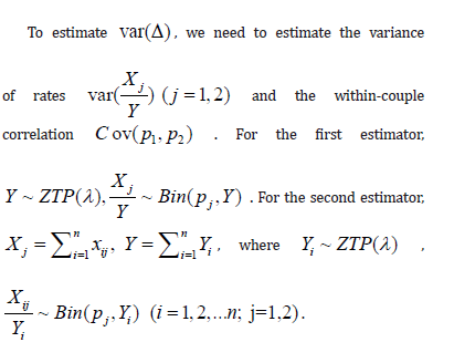
To construct the framework, we use the in vitro fertilization trial as an example for describing the motivation and setting. Let X_j be the number of high-quality euploid biastocysts (HQEB) out of Y_j mature oocytes with j^th IVF procedure, where exp-IVF (j=1) or std-IVF (j=2) We assume that 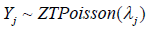zero-truncated Poisson and 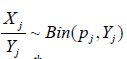where p_j is the HQEB rate (success rate) for j^th IVF procedure, respectively. Here, we assumed that the HQEB eggs are conditionally independent.

Let be the HQEB rate observed for i^th couple with exp-IVF (j=1) or std-IVF( j=2). There are two ways of estimating the HQEB rate p_j.

i.First approach: an equally average the individual rates.

ii. Second approach: 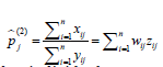a weighted average of the individual rates with weights .

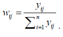It can be seen, both are unbiased estimators, i.e., The first estimator is a Least-Square Estimator (LSE), whereas the second estimator is a Maximum Likelihood Estimator (MLE). We are interested in comparing the HQEB rates with exp-IVF with std-IVF. We form a one-sided hypothesis test: 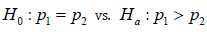Denote the treatment difference by .

Conventionally, {z_ij} is treated as normally distributed samples and analyzed with paired t-test or ANOVA. Let us call it the Conventional Approach. This approach may be appropriate when sampling size is large [7]. In this approach, the point estimate for the rate is the same as the first approach . However, there are some problems with this approach. First, it totally ignores the dependence of (cases) and Y (trials). Second, the normality condition may not be met due to skewness caused by smaller clusters (smaller denominators). As can be seen from the plots below, the departure from normality is obviously observed when λ is small. However, it is closer to normal when λ become larger (Figure 1).

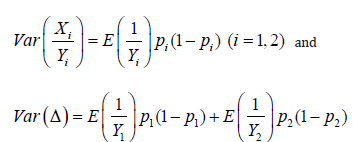
Without loss of generality, we assume i.e., equally splitting the samples within a couple. The rates can be estimated by either of the two approaches defined above. Let us discuss the variance of Δ . Note that 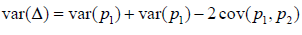.(1)

Let us drop the treatment index for a moment. Note On the other hand, since within-couple samples (matured eggs and sperms) was treated with experimental process and standard process, are correlated. Note that 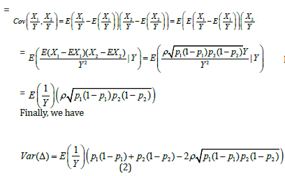It is worth mentioning that the variance for conventional approach is

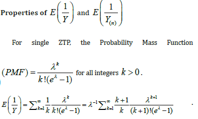
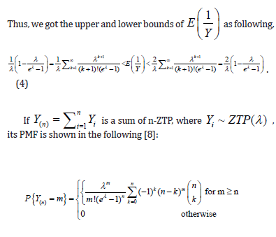
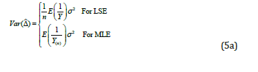
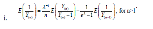
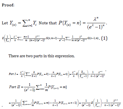
Now, the problem becomes to estimate , where Y is a single ZTP for the first approach, whereas Y is a sum of n ZTP for the second approach. Let us discuss the estimation of in the following.

Comment 1:

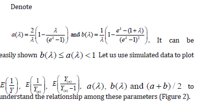
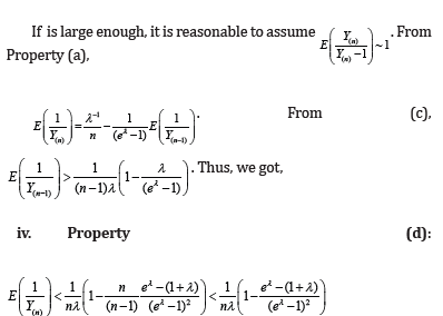
i. In property (d), we assumed when n is large. Since is the sample size (couples) of the trial, the assumption is reasonable. The orange line shows that is indeed near 1.

ii. The black solid line is which is completely bounded by a(λ).

iii. The red solid line is which is closely fitted by b(λ) .

iv. Sometimes, we saw 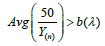slightly in the figure because may not exactly equal to 1.

v. As can be seen, is always below indicating that MLE could be more efficient than LSE. However, it could have a higher chance of Type I error inflation. Since there is a big space between a(λ) and b(λ), we use in practice to mitigate the potential Type I error inflation.

Solve λ from mean μ of ZTP

In practice, we have samples . But we need to estimate through sample mean of {y_i}. Note that the mean of ZTP is . For a given mean μ, λ can be solved numerically from equation Note the function f(λ) has maximum value at . The maximum value is 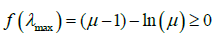. On the other hand, . So, we can numerically search for the solution in the interval of simple R function is given in the Appendix B.

Construct the Test Statistics

Recall that are the within-couple HQEB rates for exp-IVF and std-IVF, respectively. The rates can be estimated by either of the two estimators defined above. The variance of the estimators is given in the following

For the same reason, we could expect smaller sample size when using second estimator (MLE) than the first one.

Comment 2:

i. In both approaches, there are two factors that could influence the variance of treatment effect: (a) the positive correlation within-cluster, which is an uncontrollable intrinsic factor; (b) the factor a(λ) for LSE case or c(λ) for MLE case, which is a controllable extrinsic factor contributed by experimental design. From Eq. (5b), the effect size could be increased by taking the variability of the denominator into account.

ii. For both approaches, it can be seen, . The λ reflects the sampling size. If . This leads to a design strategy. We could qualify patients by requiring a minimum size of sampling (i.e., Y_j). For example, we could require that a couple to be eligible for enrollment if they produce at least 2 mature oocytes during the ovarian stimulation phase. For the colon cancer prevention study, we could enroll patients with at least 2 polyps at baseline and follow up the appearance of adenomatous polyps after a year-long prevention program.

Simulations

We conducted a simulation study to assess the ability of Type I error control and performance of attaining statistical power. For each case, 30 subjects were simulated, and 10,000 simulations were performed.

(Table 1) is a summary for assessing the Type I error inflation. The following points are observed.

Note: we set for evaluating the type I error.

i. Approaches II performed very well in Type I error control.

ii. There were some isolated cases (when λ =1 or 2) where slight inflation was seen in Approach I. However, the overall type I errors were well controlled with negative mean inflation.

iii. The conventional approach caused some type I error inflation in all cases with mean inflation of 0.0053. This could be another alarming fact for treating the rate data as normal, beside the departure from normality when λ is small as pointed earlier (Table 1).

(Table 2) summarizes the simulation results for comparing power. Since there were type I error inflation for the conventional approach, we adjusted the critical value by using , where α_I is the mean inflation rate observed in (Table 1). Please note that the baseline power is when ρ=0 and λ=1. For example, when corresponds to about 40% power. The following points are observed.

i. All approaches reached the target power.

ii. The simulated power increased as λ or ρ increased. Please note that the actual sample size for statistical tests is in fact roughly nλ. As pointed out earlier, λ is a controllable factor by design. We could increase λ to achieve higher statistical power or lower the number of subjects for achieving a target power.

iii. Baseline power for both ZTPB approaches was higher than the conventional one indicating that more efficiency could be attained if ZTPB approach was used.

iv. Approach II performed best in all cases.

Applications

We apply the ZTPB model to an in vitro fertilization (IVF) clinical trial that compares two different sperm treatment procedures. There were 81 eligible couples (age: 24-46 years old) enrolled in the study. Within each couple, female partner underwent an ovarian stimulation treatment to produce oocytes. A total of 1049 oocytes were harvested. Half of the viable oocytes will be inseminated using the male’s sperm prepared with the experimental in vitro fertilization (exp-IVF) procedure, and the other half will be inseminated using sperm prepared with the standard IVF procedure (std-IVF). The average per-couple oocytes to exp-IVF or std-IVF were 6.52 and 6.48, respectively. The primary endpoint is the rate of High-Quality Euploid Blastocysts Rate (HQEB) defined as the number of HQEBs divided by the number of mature oocytes (Tables 3-5).

The result was not significant for original analysis (pared t-test) as well as for ZTPB approaches. With the same difference in rates, however, the results could become significant by increasing λ (the sampling size). The larger the λ is, the more likely to be significant. For a study with subjects (couples), a total of samples to be studied is in fact nλ. Therefore, taking the sampling contribution into account could improve trial efficiency.

Discussion

We proposed ZTPB model for design and analysis of trials with sampling and rates. This type of design could be useful in studies with subject as sampling unit. We have demonstrated that the model is able to control the Type I error. Under ZTPB, the sampling size of each unit makes contribution to the total study samples (nλ). Therefore, it could improve the study efficiency. It could be in particularly useful for trial with rare disease where recruiting enough subjects is difficult.

We also propose two ways for estimating rates: LSE and MLE and demonstrated that MLE could be more efficient than MLE. We also demonstrated that the MLE approach performed best in term of type I error control as well as attaining higher statistical power.

In Section 2, we assumed , i.e., equally splitting the samples within a couple. This assumption can be relaxed for more general cases where the treatments or procedures begin at the stage of sample production. For example, several studies have been published for comparing procedures consisting of ovarian stimulation and sperm treatment for couples with poor ovarian response [9-11]. In this case, Y₁ and Y₂ represent oocytes produced by two different procedures on different group of couples. They are independent truncated-Poisson with different Poisson rates λ₁ and λ₂, and ρ= 0. Thus, following the similar setup as in Section 2, we get

References

- Tailiang Xie, Mikel Aickin (1997) A truncated Poisson regression model with applications to occurrence of adenomatous polyps. Statistics in Medicine 16: 1845-1857.
- Gang Li, Yifang Wu, Wenbin Niu, Jiawei Xu, Linli Hu, et al. (2020) Analysis of the Number of Euploid Embryos in Preimplantation Genetic Testing Cycles with Early-Follicular Phase Long-Acting Gonadotropin-Releasing Hormone Agonist Long Protocol. Frontiers in Endocrinology11: pp. 424.
- Linli Hu, Bo Sun, Yujia Ma, Lu Li, Fang Wang, et al. (2020) The Relationship Between Serum Delta FSH Level and Ovarian Response in IVF/ICSI Cycles. Frontiers in Endocrinology 11: pp. 536100.
- Jun Zhu, Jens C Eickhoff, Mark S Kaiser (2003) Modeling the Dependence between Number of Trials and Success Probability in Beta-Binomial-Poisson Mixture Distributions. Biometrics 59: 955-961.
- Renjun Ma, Bent Jorgensen, Jon Douglas Willms (2009) Clustered binary data with random cluster sizes: a dual Poisson modelling approach. Statistical Modelling 9(2): 137-150
- Suisui Che, Kai Huang, Jie Mi (2016) Inference about parameters in Binomial-Poisson distribution with additional incomplete data. Communications in Statistics - Theory and Methods 45(11): 3206-3222.
- Jakobsen JC, Tamborrino M , Winkel P , Haase N , Perner A, et al. (2015) Count Data Analysis in Randomised Clinical Trials. Journal of Biometrics & Biostatistics 6(1): pp. 227.
- Johan Springael, Inneke van Nieuwenhuyse (2006) On the sum of independent zero-truncated Poisson random variables. Working Papers, University of Antwerp, pp. 16.
- Linli Hu , Zhiqin Bu , Yihong Guo , Yingchun Su , Jun Zhai, et al. (2014) Comparison of different ovarian hyperstimulation protocols efficacy in poor ovarian responders according to the Bologna criteria. International Journal of Clinical and Experimental Medicine 7(4): 1128-1134.
- Ruth Howie and Vanessa Kay (2018) Controlled ovarian stimulation for in-vitro fertilization. British Journal of Hospital Medicine 79(4): 194-199.
- Li Hong Wei , Wen Hong Ma , Ni Tang , Ji Hong Wei (2016) Luteal-phase ovarian stimulation is a feasible method for poor ovarian responders undergoing in vitro fertilization/intracytoplasmic sperm injection-embryo transfer treatment compared to a GnRH antagonist protocol: A retrospective study. Taiwanese Journal of Obstetrics & Gynecology 55(1): 50-54.