


Monte Carlo Approach to Genotype by Environment Interaction Models
Oyamakin S Oluwafemi* and Durojaiye M Olalekan
Department of Statistics, University of Ibadan, Nigeria
Submission: February 08, 2020; Published: February 26, 2020
*Corresponding author: Oyamakin S Oluwafemi, Department of Statistics, University of Ibadan, Biometry Unit, Faculty of Science, Nigeria
How to cite this article: Oyamakin S Oluwafemi, Durojaiye M Olalekan . Monte Carlo Approach to Genotype by Environment Interaction Models. Biostat Biom Open Access J. 2019; 10(1): 555777. DOI: 10.19080/BBOAJ.2020.10.555777
Abstract
Understanding the implication of Genotype-by-Environment (G×E) interaction structure is an important consideration in plant breeding programs. Traditional statistical analyses of yield trials provide little or no insight into the particular pattern or structure of the G×E interaction. In this study, efforts were made to solve these problems under different level of data occurrence. We employed the simulation process of Monte Carlo in generating since use of a real-life data may pose a serious difficulty. In this paper, we simulated for two data Types of Balance and Unbalance designs with different Levels of generations (33×,77×, 1010× and 37×, 73× , 710× , 107×respectively). We therefore check the performance of interaction on four different models (AMMI, FW, GGE and Mixed model), and also their stability and adaptability. The findings revealed that, when the assumption was maintained, AMMI outperformed Finlay-Wilkinson model, GGE Biplot model and Mixed model.
Keywords: Genotype-by-Environment Interaction; Plant breeding; Stability and adaptability AMMI; FW; GGE; Mixed model; Monte Carlo Experiment
Introduction
Food insecurity is a big challenge in Africa [1]. Sub-Saharan Africa is the only region in the world currently facing both widespread chronic food insecurity and threats of famine [2]. This challenge can be addressed through focusing on a crop that requires low input and at the same time can meet major nutritional needs of the people in this region.
Genotype-by-environment interaction (GEI)
Multi-location trials play an important role in plant breeding and agronomic research. A number of parametric statistical procedures have been developed over the years to analyze genotype by environment interaction and especially yield stability over environments. A number of different approaches have been used to describe the performance of genotypes over environments. Therefore, the function that described the phenotypic performance of a genotype in relation to an environmental characterization is called the “norm of reaction” (Figure 1) shows the case where there is no GEI, the genotype and the environment behave additively (this will be developed later) and the reaction norms are parallel. The remaining plots show different situations in which GEI occurs divergence (Figure 1B), convergence (Figure 1C), and the most critical one, crossover interaction (Figure 1D). Crossover interactions are the most important for breeders as they imply that the choice of the best genotype is determined by the environment. Crossa [3] pointed out that data collected in multi-location trials are intrinsically complex having three fundamental aspects: structural patterns, nonstructural noise, and relationships among genotypes, environments, and genotypes and environments considered jointly.

Plant Breeders generally agree on the importance of high yield stability, but there is less accord on the most appropriate definition of “stability” and the methods to measure and to improve yield stability [4] tested six spring wheat cultivars at five locations across Manitoba and Saskatchewan over two years to examine genotypic and environmental variation in grain, flour, dough and breadmaking characteristics. They reported that the relative magnitude of the environmental contribution to wheat variance, depending on the trait (including yield), was considerably larger (14 to 89%) than the variance contribution of either genotype (0 to 33%) or G x E interaction (0 to 17%). Rodrigues, Monteiro & Lourenco [5] also reviewed the performance of the robust extensions of the AMMI model is assessed through a Monte Carlo simulation study where several contamination schemes are considered. Applications to two real plant datasets are also presented to illustrate the benefits of the proposed methodology, which was broadened to both animal and human genetics studies. The general aim of this study is to determine which of these models’ best suit GEI using Monte Carlo simulated data. The specific objectives are:
(i) to compare the various statistical methods and determine the most suitable parametric procedure that best describe genotype performance under multi-location trials,
(ii) to determine the efficiency of each method (AMMI, Finlay- Wilkinson, GGE and Mixed model) in detecting GEI and
(iii) Also, to determine the adaptability and specificities of the methods.
Materials and Methods
A combined analysis of variance procedure is the most common method used to identify the existence of GEI from replicated multi-location trials. If the GEI variance is found to be significant, one or more of the various methods for measuring the stability of genotypes can be used to identify the stable genotype(s). A wide range of methods is available for the analysis of GEI and can be broadly classified into four groups: the analysis of components of variance, stability analysis, multivariate methods and qualitative methods. The methods to be adopted in this study are suitable for the plant breeders in estimating Genotype by Environment Interaction (GEI) parameters. The methods are as follows
AMMI model
The AMMI model combines the features of ANOVA and SVD as follows: first, the ANOVA estimates the additive main effects of the two-way data table; then the SVD is applied to the residuals from the additive ANOVA model, estimating interaction principal components (IPCs). The model can be written as [6].

where ijk y is the phenotypic trait (yield or some other quantitative trait of interest) of the ith genotype in the jth environment for replicate k;
μ is the grand mean
α are the genotype deviations from;
β are the environment deviations from;
n λ is the singular value of the IPC analysis axis n?
γ and n, j δ are the ith and jth genotype and environment IPC scores (i.e. the left and right singular vectors, scaled as unit vectors) for axis n, respectively i, j ρ is the residual containing all multiplicative terms not included in the model;
e is the experimental error; and N is the number of principal components retained in the model.
In matrix formulation the AMMI model can be written as:

where Y is the (I × J ) two-way table of genotypic means across environments. The interaction part of the model * 1T 1T 1 T I j I J I J Y = Y − μ −α − β is approximated by the product of matrices UDVT , with U an (I × N)matrix whose columns contain the left singular vectors interactions of n, D a (N × N) diagonal matrix containing the singular values of Y* , and V a (J × N) matrix whose columns contain the right singular vectors of Y*
Finlay-Wilkinson model
A more attractive alternative is to extend the additive model:

by incorporating terms that explain as much as possible of the GEI. A popular strategy in plant breeding is that proposed by Finlay and Wilkinson (1963), which describes GEI as a regression line on the environmental quality. In the absence of explicit environmental information, the biological quality of an environment can be reflected in the average performance of all genotypes in that environment. The GEI part is then described by genotype-specific regression slopes on the environmental quality, and the model can be written in the following equivalent ways:

Model (5) follows from model (4) by taking ' i i μ +α =α and (1 ) 'j i j i j i j β + bβ = + b β = b β . Model (5) is easier to interpret because it looks as a set of regression lines; each genotype has a linear reaction norm with intercept and slope. The explanatory environmental variable in these reaction norms is simply the environmental main effect j β . Model (4) shows more clearly how GEI is captured by a regression on the environmental main effect, with the hope that as much as possible of the GEI signal will be retained by the term i j bβ . Note that in model (5) the average value of b' is 1, meaning that b' >1 for genotypes with a higher than average sensitivity, and b' <1 for genotypes that are less sensitive than average [7,8].
GGE model
Plant breeders are interested in the total genetic variation and not exclusively in the GEI part. For that reason, it is useful to have a modification of model (1) that considers the joint effects of the genotypic main effect and the GEI as a sum of interpretation procedures hold as for model (1). Because genotypic scores now describe genotypic main effects G and GEI together, this type of model is also known as the “GGE model” and the Biplots are called “GGE Biplots”. The model reads:

In GGE, the result of SVD is often presented in a “Biplot illustration”. Its approximate overall performance (G + GEI).
Mixed model
The REML/BLUP method allows the consideration of different structures of variance and covariance for the genotypes by environments effects, which makes the model more realistic. For the GEI evaluation by mixed model, the following statistical model was used:

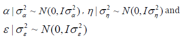
Where, y is the vector of observed data; is the vector of genotype effects (assumed as random); β is the vector of block effects within each environment (assumed as fixed); η is the vector of GEI effect (assumed as random); and ε is the error vector (random). The uppercase letters represent the matrices of incidence for the referred effects. The distribution of the random effects were:
Setting up Monte Carlo Experiment
We simulate two-way data tables for balanced and unbalanced design with 3 replications each, where the interaction is explained by two multiplicative terms (i.e. two IPCs; k = 2 components to be retained). Without loss of generality, the two-way data tables are simulated in the following way:
Balance design
a) Create a matrix X with (n× p) data design
b) (3×3) data design, where n = 3 rows (Genotypes) and p = 3 columns (Environments)
c) (7×7) data design, where n = 7 rows (Genotypes) and p = 7 columns (Environments).
d) (10×10) data design, where n = 10 rows (Genotypes) and p = 10 columns (Environments).
e) with observations drawn from a Unif [0, 0.5] distribution.
f) Do the SVD of X and obtain the matrices U, V and D, containing, respectively, the left and right singular vectors and the singular values of X.
g) Simulate the grand mean, the genotypic and environmental main effects, considering: μ ~ N(15,3) α ~ N(5,1) and β ~ N(8, 2) (Rodrigues et al.(2015)).
Unbalanced design
a) (n× p) Create a matrix X with data design.
a. (3×7) data design, where n = 3 rows (Genotypes) and p = 7 columns (Environments)
b. (7×3) data design, where n = 7 rows (Genotypes) and p = 3 columns (Environments).
c. (7×10) data design, where n = 7 rows (Genotypes) and p = 10 columns (Environments).
d. (10×7) data design, where n = 10 rows (Genotypes) and p = 7 columns (Environments).
e. with observations drawn from a Unif [0, 0.5] distribution.
f. Do the SVD of X and obtain the matrices U, V and D, containing, respectively, the left and right singular vectors and the singular values of X;
g. Simulate the grand mean, the genotypic and environmental main effects, considering: μ ~ N(15,3) α ~ N(5,1) and β ~ N(8, 2) [5].
Results and Discussion
Model stability and adaptability
a. Balance design: Comparison of stability of different models using different stability parameters (Table 1) shows the model stability for balance design of which we observed that among all the models, AMMI and FW are the most stable models for simulated design showing the highest stability ranked mean of 24.18 and regression coefficient deviation from 1 respectively. Similarly, on the same table, GGE and mixed model claimed to be stable at simulated design. That is, the complete GGE model contained 98.5% of the Sum of Square, and the residual 1.5%. Also, the Mixed Model showed the lowest ranked stability variance (i.e. σ 2 =1.919 ). The biplot analysis system showing in (Figure 2) are the visual inspection plots that show the most adap\ models. Therefore, it was observed that the closer the concentric circles to the center point, the more adaptable the models. Similarly, in the second plot, the closer the model to the thick blue arrow line, the more adaptable the model. It can be deduced that from the balance design simulated data, AMMI model is more stable and better adaptable.


b. Unbalance design: Comparison of stability of different models using different stability parameters (Table 2) shows the model stability for Unbalance design of which we observed that among all the models, AMMI and FW are the most stable models for simulated design showing the highest stability ranked mean of 24.5 and regression coefficient deviation from 1 respectively. Similarly, on the same table, GGE and mixed model claimed to be stable at and simulated design. That is, the complete GGE model contained 94.5% of the Sum of Square, and the residual 5.5%. Also, the Mixed Model showed the lowest ranked stability variance (i.e. 228.19σ=). In the same vein, the biplot analysis system showing in (Figure 3) are the visual inspection plots that show the most adaptable models. Therefore, it was observed that the closer the concentric circles to the center point, the more adaptable the models. Similarly, in the second plot, the closer the model to the thick blue arrow line, the more adaptable the model. It can be deduced that from the Unbalance design simulated data, AMMI model is more stable and better adaptable.
Model evaluation for simulated data
(Table 3) displayed the comparison of the four models using model evaluation criterion (RMSE, MSE and Absolute Bias). However, across all the simulated data for balance design, AMMI model is consistent at the minimum values for RMSE and Absolute Bias (i.e. very close to the true parameters). Except at 1010× data design where mixed model revealed minimum value at MSE criteria. More so, Unbalance design on the same table observed similar report across different level of design that AMMI is still influential. Except at 37×data design where mixed model revealed minimum value at MSE criteria.


Conclusion
In this study, efforts were made to solve these problems under different level of data occurrence. We employed the simulation process of Monte Carlo in generating since use of a real-life data may pose a serious difficulty. In this research work, we simulated for two data Types of balance and unbalance designs with different Levels of generations (33×,77×, 1010× and 37×, 73× , 710× , 107×respectively). The findings revealed that, when the assumption was maintained, AMMI outperformed Finlay-Wilkinson model, GGE Biplot model and Mixed model. We therefore check the performance G×Eof interaction on four different models (AMMI, FW, GGE and Mixed model), and their stability and adaptability. Finally, the study has clearly shown that the four models considered detects the G×E interaction effect in a different way. We were able to evaluate and described interaction performanceG×E by their stability and adaptability using multi-location trials. Also, this study confirmed the suitability of AMMI in detectingG×E when the assumptions are maintained or kept. That is, when outlier is not influential, AMMI can be used.
Implementation
Phase II trials, especially adaptive designs, require close collaborations among all staff in the study team. The study team includes the physician/PI, biostatistician, data manager/coordinator, research nurses and IT support. The communication among all staff is key to have a robust design and implementation of the trial. While many practical considerations are like traditional designs and advanced adaptive designs, additional considerations may be required for particular types of adaptive designs [18]. First, these more advanced designs require additional planning time to select the proper endpoint(s) and obtaining preliminary data. Adaptive designs are usually more complicated than the traditional designs. Simulations are needed to help interpreting and understanding the operation characteristics curve of the adaptive design. Second, prior to the trial initiation, all team members need training on the logistical aspects of the trial, and the team should know the communication matrix during the trial. The training is essential to minimize errors and ensure the successful implementation of the trial. Third, interim analyses or adaptive procedures, which should be clearly stated in the protocol, need to be conducted timely at the designated time. This requires consistent data monitoring and quality checking throughout the trial duration, and the statistician needs to be readily prepared to work on all the analyses. These additional efforts should be considered in the study budget and the planning process. Prior to obtaining funding to run the trial, institutional support should be provided to support investigators team on the pre-planning process. Each adaptive trial design could be implemented slightly differently depending on the available resources/infrastructure of each institution.
Conclusion
As we have discussed, several aspects need to be considered to choose a proper statistical design: single arm versus randomized trial, traditional design versus adaptive design. The background of the disease type and patient population as well as the preliminary data are all critical elements for Phase II clinical trial designs. While more advanced adaptive designs have been proposed to improve the operation characteristics over the traditional designs, PIs should be provided with the opportunity to learn about these designs and build trust with the biostatistician and the rest of the research team on the implementation process. Institutional support and infrastructure are the most critical aspects for the successful designing and implementation of investigator initiated clinical trials in academic medical centers.
Funding Support
All authors were partially supported by the National Institutes of Health / National Center for Advancing Translational Sciences grant UL1TR002733 and OSU Comprehensive Cancer Center Support Grant P30CA016058.
References
- UNESCO (2009) Economic Commission for Africa. Committee on Food Security and Sustainable Development. Sixth Session. Regional Implementation Meeting for CSD-18. The Status of Food Security in Africa.
- Devereux S, Maxwell S (2001) Food Security in Sub-Saharan Africa. ITDG Publishing.
- Crossa J (1990) Statistical Analyses of Multilocation Trials. Advances in Agronomy 44: 55-85.
- Finlay GJ, Bullock PR, Sapirstein HD, Naeem HA, Hussain A, Angadi SV (2007) Genotypic and environmental variation in grain, our, dough and bread-making characteristics of western Canadian spring wheat. Can J Plant Sci 87: 679-690.
- Rodrigues PC, Andreia M, Vanda ML (2015) A robust AMMI model for the analysis of genotype-by-environment data. Bioinformatics 32(1): 58-66.
- Gauch HG (1988) Model selection and validation for yield trials with interaction. Biometrics Pp. 705-715.
- Finlay KW, Wilkinson GN (1963) The Analysis of Adaptation in a Plant breeding Program Pp. 742-54.
- Gauch HG (2006) Statistical Analysis of Yield Trials by AMMI and GGE. Crop Science 46: 1488-1500.


