


Linear Quantile Regression and Endogeneity Correction
Christophe Muller*
Faculty of Economics and Management, Aix-Marseille University, France
Submission: July 19, 2019; Published: August 26, 2019
*Corresponding author: Christophe Muller, Faculty of Economics and Management, Aix-Marseille University, CNRS, EHESS, Ecole Centrale, IRD, AMSE, Marseille, France
How to cite this article: Christophe Muller. Linear Quantile Regression and Endogeneity Correction. Biostat Biom Open Access J. 2019; 9(5): 555774. DOI: 10.19080/BBOAJ.2019.09.555774
Abstract
The main two methods of endogeneity correction for linear quantile regressions with their advantages and drawbacks are reviewed and compared. Then, we discuss opportunities of alleviating the constant effect restriction of the fitted-value approach by relaxing identification conditions.
Keywords: Two stage estimation; Quantile regression; Fitted-Value Approach; Endogeneity
Abbreviations: TLS: Trimmed Least Squares; LAD: Least Absolute Deviations; CDF: Cumulative Distribution Function; PDF: Probability Density Function
Introduction
Endogeneity issues in regression models have been well studied in econometrics, though they may have been less fully investigated in the biometric and biostatistic literature. Endogeneity in regression model estimation may arise from reverse or feed-back causality, correlated measurement errors in dependent and independent variables, and unobserved heterogeneity correlated with dependent and independent variables.
It is not difficult to find examples in which endogeneity is a problem in biological sciences. For example, in observations of natural phenomena in biological sciences, the presence of an unobserved variable correlated with both the dependent and independent variables is often likely to generate endogeneity biases in regression estimates. Consider for instance the study of infant weights in some tropical country. In this context, heavy rains can simultaneously cause higher travelling costs because of flooded roads, on the one hand, and, worse health status, because of malaria spurred by a larger number anopheles mosquitoes, on the other hand. Then, lower observed weights may result from higher malaria incidence. However, it may also come from inefficient health care delivery caused by transportation delays. In that case, in a regression of observed infant weights on malaria spells, one expects some endogeneity of this latter variable associated with unobserved transport costs. Moreover, information on rains can be used an instrument for malaria
In this example, investigating low quantiles of baby weights, and not only the mean weight, is crucial as these weights are ex cellent measures of child nutrition status, and what matters is that the weight does not fall under a minimal threshold.
More generally, analyzing distributions of outcomes in biological or medicine studies is fundamental as the global average may hide many interesting and vital phenomena. Quantile regressions have been found a convenient statistical tool for such explorations and for better understanding the heterogeneity of the observed individual units in general. The practical statistical use of quantile regressions was popularized by Bassett & Koenker [1] and Koenker & Bassett [2] who brought to the fore tractable computational techniques and derived asymptotic properties for these methods.
Quantile regressions allow for any given regressor having different effects for different individual units. Therefore, using quantile regressions increases the flexibility of the models. It also enables researchers to explore specific locations of the conditional distribution of the outcome variable, in particular the lower and upper tails. In that case, more substantial explanations of the variability of the studied phenomenon can be obtained, particularly in the case of nonconstant effect; that is with regression coefficients varying across quantiles.
Different approaches have been pursued for dealing with endogeneity issues in quantile regressions. On the one hand, an analogue of the instrumental regression approach, based on exclusion restrictions, has been developed by Chernozhukov and Hansen [3-6]. It is associated with specifications of the conditional quantile function of main equation of interest.1 It allows for nonconstant quantile effects.
On the other hand, the fitted-value approach corresponds to another analogue of the typical two-stage least-square estimator for quantile regression. It was pioneered by Amemiya [7] and Powell [8] who laid their theoretical properties for two-stage least-absolute-deviations estimators in a simple setting. First, fitted-values of the endogenous regressors are estimated using a set of exogenous independent variables. Then, the estimation of the quantile regression of interest is performed by substituting the endogenous regressors with their fitted-values. This approach can be seen as imposing restrictions on the quantile of the reduced-form error. It makes sense to pay particular attention to reduced-form equations in experimental settings or policy design. Blundell & Powell [9] pointed out that the reduced-form is of interest when control variables for the policy maker include instrumental variables. In social statistics, the pro-poor targeting of social programs can be improved by relying on predictions of living conditions based on well focused quantile regressions of reduced forms [10,11]. Similarly, in public health interventions, predictive quantile equations of health outcomes are useful; and so on for other biological sciences in which targeting interventions may be important.
Using this approach, Chen [12] and Chen & Portnoy [13] studied two-stage quantile regression in which trimmed least squares (TLS) and least absolute deviations (LAD) estimators are employed as the first-stage estimators. To reduce the variance of two-stage quantile regression estimators, Kim and Muller [14] constructed a weighted average of the dependent variable with its fitted value from a preliminary estimation, which is employed as the dependent variable in a final two-stage quantile regression. Kim and Muller [15] used a similar approach with instead quantile regression in the first stage. We now turn to a more precise discussion of the conditions in which these estimation methods yield consistent estimation and other useful properties.
Results and Discussion
Models and assumptions
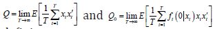
Let us consider the estimation of the parameter

where
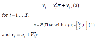
By assumption, the following linear equation, which is assumed to be correctly specified, can be used to generate an exogenous fitted-value for :tY

where []12,tttxxx′′′= is a K row vector with 12.KKK=+ Matrix Π is a KG× matrix of unknown parameters, while tV′ is a G row vector of unknown error terms. Assumptions 2 and 4 below will complete the DGP. However, let us first discuss the reduced form.
Using (1) and (2) yields:
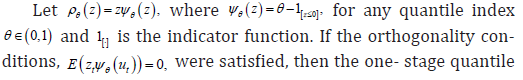
The Two-Stage Quantile Regression estimator ˆαof αis defined, for any quantile ,θ as a solution to:

where ˆΠ is a first-stage estimator. Let us state a few hypotheses and regularity assumptions.

This is the main identifying condition of the fitted-value approach with quantile regression.
i. Assumption 3: (i) ()HBΠΠ+ is of full column rank.
(ii) Let ()tFx⋅ be the conditional cumulative distribution function (CDF) and ()tfx⋅ be the conditional probability density function (PDF) of .tv The conditional PDF ()tfx⋅ is assumed to be Lipschitz continuous for all ,x strictly positive and bounded by a constant 0f (i.e., ()0,tfxf⋅< for all x).
(iii) The matrices
(iv) There exists 0,C> such that
In Kim and Muller, a general asymptotic expansion is derived that can be used to compute the particular case in the following theorem by plugging the asymptotic expansion of a first stage OLS estimator ˆΠ in it, to obtain:
Theorem 1
Under Assumptions 1-3, the asymptotic representation for the two-stage quantile regression estimator is:
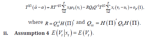
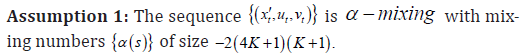
1. Assumption 4 imposes the independence of the reduced-form errors with all non-constant exogenous variables and it corresponds to the use of unbiased OLS in the first stage.
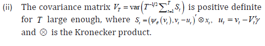
iii. Assumption 5
(i) There are finite constants ,Δ such that

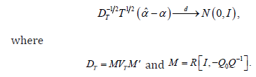
Theorem 2
Under Assumptions 1-5 [14],
Therefore, calculating the estimator and performing asymptotic inference is straightforward with this approach. In contrast, the instrumental variable approach in that case assume, instead of Assumption 2, that the conditional quantile of tu with respect to
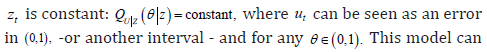
Specifically, the IV-QR estimator of the coefficient vector for the endogenous regressors is
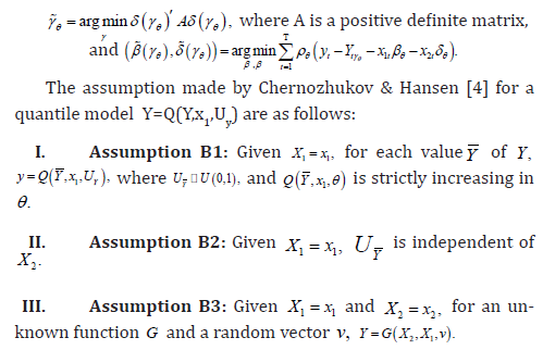
IV. Assumption B4: For any values Y and ,Y′ given ()12,,,
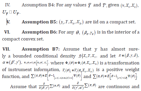
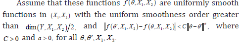
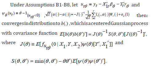
VIII. Assumption B8: Almost surely, the following estimated function, denoted ()12,,,fXXθ converge in probability uniformly in ()12,,XXθ over compact sets: ()12,,XXθΦ and ()12ˆ,,.
Theorem 3
Let us now compare the two approaches in the next subsection.
Advantages and drawbacks of the two approaches
On the one hand, the fitted-value approach is often convenient. It corresponds to an elementary OLS and quantile regressions, which is practically analogous to the two-stage least-square procedure. For this reason, it has been used by empirical researchers keen to avoid computation problems.2 In particular, no non-parametric estimation, no simulations, no numerous iterations of computation steps nor optimisation grid are needed. The fitted-value approach also allows the use of a new method of variance reduction for quantile regressions proposed by Kim & Muller [14] under very general conditions.

In contrast, an issue with the IV approach is that it may be costly in terms of numerical computations to perform. extracted from the following table, extracted from Kim & Muller (2018) [30] compares computation times using the fitted-value approach in Kim & Muller [14,15] and the Chernozhukov & Hansen [3] procedure and programs, for a simple simulation setting Table 1.
The computation time for the Chernozhukov and Hansen test is much higher because of the iterations for the numerical approximation of the first-order conditions, especially with more than one endogenous regressor. Although this drawback may be alleviated by using more efficient algorithms, it remains an issue when there are many endogenous regressors.
However, recently, new codes and methods have been developed by Kaplan and Sun (2017) and de Castro, Galvao, Kaplan and Lin (2020) that are just faster, and therefore offer a promising avenue of development.
On the other hand, the fitted-value approach is often plagued by the occurrence of constant effects, as claimed by Lee [17]. That is: all coefficients, except for the intercept, should be the same for all considered quantiles, which makes the model less flexible and therefore less realistic. However, even if this drawback is real, this is not completely so. Muller [18] showed that it is possible to estimate two-stage quantile regressions using the fitted-value approach that are consistent with a particular form of nonconstant effects. In that case, heterogeneous coefficients can be allowed for some of the model regressors only. This can be obtained by assuming weaker instrumental variable restrictions than usual. Under these weakened conditions, the endogeneity can be treated by using the fitted-value approach, although the nonconstant effects have to correspond to parameters that are in the model but cannot be identified precisely. However, nonconstant effects, varying with the quantile index, can still be present in the true model. Another shortcoming of the fitted-value approach is that the first-stage equation must be well specified, whereas this is not required for the instrumental variable approach.
However, there is also some common ground between the two approaches. Indeed, even under constant effects, quantile regressions can be useful when only one given quantile is of interest, for example when the considered intervention or experiment is targeted to this quantile. In that case, both methods are appropriate. Moreover, when one is only interested in the individual mean, then the two approaches can be seen as equivalent under exact identification [19].
Relaxing identification conditions
The above-mentioned interest in relaxing identification requirements for quantile regression under endogeneity invites to pursue the discussion in this direction. Assumption 2 imposes that zero is the given thθ-quantile of the conditional distribution of ,tvθ where the quantile index θ has been added to tv to show well that Assumption 2 characterizes a given quantile index .
iv.
Assumption 6: For a given quantile index ,θ the cdf of tvθ conditional on ,tx denoted ,ttvxFθ the cdf of tvθ conditional on 1,tx denoted 1,ttvxFθ and the marginal cdf of x2t, denoted x2t
Now, instead of Assumption 2, the weaker Assumption 2’can be used. Assumption 2’: For a given quantile θ and under Assumption 1: tvθis independent of x2t, conditionally on 1.tx (6) In Muller, it is shown that Theorem 4: (Chernozhukov and Hansen): Under Assumptions 18, 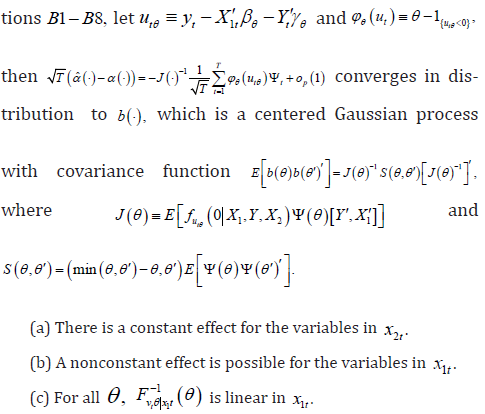
(a) There is a constant effect for the variables in 2.tx (b) A nonconstant effect is possible for the variables in 1.
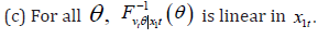
The popular ‘linear location-scale hypothesis’ in the quantile regression literature on the non-constant effect (e.g., Koenker [20]) is consistent with Result (c) in Proposition 1. Moreover, Result (c) may be easily relaxed by including polynomial terms in x1t in the model. Alternatively, the reduced form in (3) could be specified as being partially linear in x2t, and nonlinear in 1,tx with an unknown nonlinear functional form. This still yields a constant effect for 2txand an unrestricted nonlinear effect for 1.tx In that case, Result (c) could be discarded. Finally, instead of imposing Assumption 2, one may first test for which coefficients the hypothesis of constant effect is rejected or not in typical quantile regression estimation, so as to guide the precise specification of this assumption. Finally, the results in Muller [30] are:
Theorem 5
Under Assumptions 1 and 2:
(a) The components of θπ in the reduced form (3) for any quantile index θ can be identified, for the constant coefficients
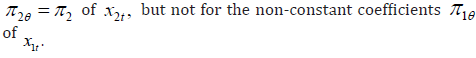
(b) For the quantile model (1), the coefficient vector θγ of the endogenous regressors tY in the quantile model is identified, while constant with respect to the quantile index :,θθγγ= for all ()0,1.
(c) The coefficient vector θβ of the exogenous regressors x1t in the quantile model can be non constant with respect to the quantile index ,θ while it is not identified in general.
In biological sciences, obtaining a condition like in Assumption 2, or a similar one by reversing the roles of x1t and x2t, should be much easier than in social sciences. Indeed, experimental settings or specification of controls could be designed accordingly
Conclusion
The design of identification conditions for solving endogeneity issues in quantile regressions is still an open research area. The diverse methods used in the literature to deal with the problems discussed here correspond to non-encompassing restrictions. It seems therefore fruitful to further investigate and develop each kind of approach. We have sketched the state of the question from which such extension could be built on.
In particular, a few reservations would deserve further investigation. First, studying some practical applications based on actual policy data or experiment data that are characterised by constant effect of treatment variables would assist in clarifying the potential of the respective methods. Second, the rigid distinction between constant effect and nonconstant effect for endogenous and exogenous regressors could be relaxed to generate more flexible specifications. Third, as always, finding instruments, even if weakened ones, is still hard in general. However, owing to controlled experiments, this may be easier in biological sciences than in other study areas.
References
- Bassett G, Koenker R (1978) Asymptotic theory of least absolute error regression. Journal of the American Statistical Association 73: 618-622.
- Koenker R, G Bassett (1978) Regression quantiles. Econometrica 46: 33-50.
- Chernozhukov V, Hansen C (2005) An IV Model of Quantile Treatment Eff Econometrica 73: 245-261.
- Chernozhukov V, Hansen C (2006) Instrumental Quantile Regression Inference for Structural and Treatment Effect Models. Journal of Econometrics 132: 491-525.
- Chernozhukov V, Hansen C (2008a) Instrumental Variable Quantile Regression: A Robust Inference Approach. Journal of Econometrics 142: 379-398.
- Chernozhukov V, Hansen C (2008b) The Reduced Form: A Simple Approach to Inference with Weak Instruments. Economics Letters 100: 68-71.
- Arias O, Hallock KF, Sosa Escudero W (2001) Individual Heterogeneity in the Returns to Schooling: Instrumental Variables Quantile Regression Using Twins Data. Empirical Economics 26: 7-40.
- Powell J (1983) The Asymptotic Normality of Two-Stage Least Absolute Deviations Estimators. Econometrica 51: 1569-1575.
- Blundell R, Powell JL (2006) Endogeneity in Nonparametric and Semiparametric Regression Models. In: Dewatripont M, et al. Chapter 8th, Advances in Economics and Econometrics: Theory and Applications, Eighth World Congress, Cambridge University Press, Pp: 312-356.
- Muller C (2005) Optimising Anti-Poverty Transfers with Quantile Regressions, Applied and Computational Mathematics 4: 2.
- Muller C, Bibi S (2010) Refining Targeting against Poverty: Evidence from Tunisia. Oxford Bulletin of Economics and Statistics 72: 3.
- Chen LA (1988) Regression Quantiles and Trimmed Least-Squares Estimators for Structural Equations and Non-Linear Regression Models, Unpublished Ph.D. dissertation, University of Illinois at Urbana-Champaign.
- Chen LA, Portnoy S (1996) Two-Stage Regression Quantiles and Two-Stage Trimmed Least Squares Estimators for Structural Equation Models. Commun Statist Theory Meth 25: 1005-1032.
- Kim T, Muller C (2018) Inconsistency Transmission and Variance Reduction in Two-Stage Quantile Estimation(with T.-H. Kim), Forthcoming in Communications in Statistics: Computation and Simulation.
- Kim T, Muller C (2004) Two-Stage Quantile Regressions when the First Stage is Based on Quantile Regressions. The Econometrics Journal 18-46.
- Kim T, Muller C (2012) A Test for Endogeneity in Quantiles, Working Paper Aix Marseille School of Economics.
- Lee S (2007) Endogeneity in Quantile Regression Models: A Control Function Approach. Journal of Econometrics 141(1): 1131-1158.
- Kim T, Muller C (2017) A Robust Test of Exogeneity Based on Quantile Regressions. Journal of Statistical Computation and Simulation 87(11): 2161-2174.
- Galvao AS, Montes-Rosas G (2015) On the Equivalence of IV Estimators for Linear Models. Economic Letters 134: 13-15.
- Koenker R (2005) Quantile Regressions, Cambridge University Press, Cambridge.
- Abadie A, Angrist J, Imbens G (2002) Instrumental Variables Estimates of the Effect of Subsidized Training on the Quantiles of Trainee Earnings. Econometrica 70: 91-117.
- Amemiya T (1982) Two Stage Least Absolute Deviations Estimators. Econometrica 50: 689-711.
- Chernozhukov V, Imbens GW, Newey WK (2007) Instrumental Variable Estimation of Nonseparable Models. Journal of Econometrics 139(1): 4-14.
- Chevapatrakul T, Kim T, Mizen P (2009) The Taylor Principle and Monetary Policy Approaching a Zero Bound on Nominal Rates: Quantile Regression Results for the United States and Japan. Journal of Money, Credit and Banking 41: 1705-1723.
- Chortareas G, Magonis G, Panagiotidis T (2012) The Asymmetry of the New Keynesian Phillips Curve in the Euro Area. Economics Letters 114(2): 161-163.
- Garcia J, Hernandez PJ, Lopez A (2001) How Wide is the Gap? An Investigation of Gender Wage Differences Using Quantile Regression. Empirical Economics 26(1): 149-167.
- Hong H, Tamer E (2003) Inference in Censored Models with Endogenous Regressors. Econometrica 71: 905-932.
- Honore BE, Hu L (2004) On the Performance of Some Robust Instrumental Variables Estimators. Journal of Business and Economic Statistics 22: 30-39.
- Ma L, Koenker R (2006) Quantile Regression Methods for Recursive Structural Equation Models. Journal of Econometrics 134: 471-506.
- Muller C (2018) Heterogeneity and nonconstant effect in two-stage quantile regression. Econometrics and Statistics 8: 3-12.
- Sakata S (2007) Instrumental Variable Estimation Based on Conditional Median Restriction. Journal of Econometrics 141: 350-382.


