Parameters Estimation of Weibull Distribution g Based on Fuzzy Data Using Neural Network
Gajendra K Vishwakarma, Chinmoy Paul* and Neha Singh
Department of Applied Mathematics, Indian Institute of Technology Dhanbad, India
Submission: February 19, 2018; Published: April 30, 2018
*Corresponding author: Chinmoy Paul, Department of Applied Mathematics, Indian Institute of Technology Dhanbad, Jharkhand-826004, India; Email: chinmoy.gcc@gmail.com
How to cite this article: Gajendra K V, Chinmoy P, Neha S. Parameters Estimation of Weibull Distribution Based on Fuzzy Data Using Neural Network. Biostat Biometrics Open Acc J. 2018; 6(5): 555696. DOI:10.19080/BBOAJ.2018.04.555696
Abstract
In this article, an estimation procedure to estimate the parameters of a two-parameter Weibull distribution has been discussed. The nature of the data is considered as imprecise and is in the form fuzzy numbers. Artificial Neural Network has been used in parameter estimation of Weibull distribution. The network architecture is determined experimentally based on RMSE. Other classical methods of parameter estimation such as method of moments, maximum likelihood estimation and Bayesian estimation are also discussed. Performances of each of these methods are compared using mean and standard deviation of the estimates based on the simulated data for a various range of parameter values
Keywords: Artificial neural network; Maximum likelihood estimator; Method of moments; Weibull distribution; Simulation; Parameters; Standard deviation; Likelihood estimation; Bayesian estimation; Rayleigh distribution; Probability density function; Cumulative distribution function; Maximization; Unexpected errors; Algorithms; Fuzzy; Imprecision; Parameter estimation; Parameter estimation; Graphical approach; Maximization step
Abbreviations: MLE: Maximum Likelihood Estimates; EM: Expectation Maximization; NR: Newton Raphson's; MSE: Mean Square Error; ANN: Artificial Neural Network
AMS Subject Classification Number: 62F15, 62F86.
Introduction
Weibull distributions have several desirable properties and these properties have nice physical interpretations. Weibull distribution generalizes exponential and Rayleigh distribution. It was W. Weibull who first introduced Weibull distribution way back in 1937 for estimating reliability and life testing of machinery. In literature, we can find Weibull distribution with three as well as two parameters. A random variable'X ' following Weibull distribution with two parameters (a,p) has following probability density function (pdf) and cumulative distribution function (cdf)

Respectively, where (αβ)>o are scale and shape parameters. The Weibull distribution is generally used in reliability modeling and life testing. The estimation of its parameters has been discussed by Qiao & Tsokos [1]. Graphical approach is generally used for its simplicity and speed. Balakrishnan & Kateri [2] have proposed a very simple and easily applicable graphical approach for parameter estimation of Weibull distribution. This approach easily shows the existence of maximum likelihood estimates (MLE). However, graphical approaches are subjected to probability of error in measurement.
Type-I and Type-II censoring is another method under which parameter estimation of Weibull distribution is discussed by several articles. Censored data usually arise in circumstances like a disease or a lack of success is only partially observed, because collection of information is done at certain examination times. Watkins [3] presented maximum likelihood estimation (MLE) approach for Weibull distribution when the nature of data for analysis contains both times to failure and censored times. Marks [4] introduced an effective iterative procedure for the estimation. Banerjee & Kundu [5] in their study, they have discussed a hybrid censoring method that is a combination of Type-I and Type-II censoring schemes. Their study presented an approach of obtaining estimates of unknown parameters iteratively. Zaindin & Ammar [6] considered modified Weibull distribution based on Type II censored data. They deal with the problem of estimating the parameters of this distribution based on maximum likelihood and traditional least square techniques.
When the explicit forms of the estimates are not readily available by directly solving likelihood functions, then the need for iterative procedure arises. Among the frequently used iterative procedures expectation maximization (EM) algorithm is very often used as far as parameter estimation of Weibull distribution is considered. Another method that is commonly used is Newton Raphson's (NR), based on numerical methods. Panahi & Saeid
[7] discussed estimation of the Weibull distribution based on type-II censored samples. When we have prior knowledge about the parameter distribution Bayesian estimation procedure can be used. Nandi & Dewan [8] have considered the problem of estimation of the parameters of the Marshall Olkin Bivariate Weibull distribution in the presence of random censoring. They used EM algorithm instead of maximum likelihood estimators as the parameters cannot be articulated in a closed form by the use of MLE. Balakrishnan & Mitra [9] considered truncation and right censoring data and EM algorithm NR methods were applied to estimate the model parameters. But all the iterative methods have shortcoming in terms of stopping criteria, time complexity and tendency to convergence locally.
In all the above inferential methods, data considered was precise in nature. But in real life situation that it is sometimes difficult to measure and record precise data. In many occasions due to unexpected errors, assignable causes or due to machine errors precise data can't be recorded. Pak et al. [10] in their study considered the problem in which parameters of Weibull distribution are estimated based on the fact that collected data is not precise and are considered in the form of fuzzy numbers. Maximum likelihood estimates (MLEs) of the parameters were obtained by Newton-Raphson (NR) and Expectation Maximization (EM) algorithms. Bayes estimates of the unknown parameters were obtained by assumption of Gamma priors. Gertner & Zhu [11] Bayesian estimators based on two kinds of extension to the fuzzy likelihood functions for a given fuzzy prior. Thierry [12] presented a method of estimating the parameters of a parametric statistical model when nature of data is fuzzy and are assumed to be related to underlying crisp realizations of a random sample.
When we discuss about iterative procedures for parameter estimation, approaches based on artificial neural network do find its place. Abbasi et al. [13] have proposed an artificial neural network based approach for estimating parameters of Burr XII distribution. Likas [14] proposed a method for density estimation based on neural network approach. Parameter estimation of K-distribution based on Method of moments, Method of maximum likelihood estimation (MLE) and neural network respectively has been discussed by Iskander et al. [15] and Wachowiak et al. [16]. We consider the problem which is different from censoring and truncation when the data for Weibull random variable is fuzzy in nature and then develop artificial neural network based approaches to estimate the parameters. Also compared results based on neural network approach with NR, EM algorithm, Bayesian approach.
Fuzzy sets and probability
Fuzzy set theory describes a calculus for the uncertainty associated with classification, or what is called as "imprecision". But it is quite possible that both uncertainty and imprecision can be present in the same problem, Zadeh [17] and Singpurwalla & Booker [18] in their study stated that "Probability must be used in concert with fuzzy logic to enhance its effectiveness. In this perspective, probability theory and fuzzy logic are complementary rather than competitive". Let Rn,P denote a probability space where A is the field of Borel sets in Rn,P is the measure satisfying 0≤P≤1 Then, the probability of an event A that is fuzzy is nature can be defined over Rn by:

Fuzzy data and likelihood function
Suppose that (x1x2 .... xn) is a sample of size n drawn randomly from the distribution with probability density function given by Eq. (1). Further suppose that the corresponding random vector be denoted as x = (x1,x2....xn). If any realization x = (x1,x2....xn) of X was known precisely, we could find the likelihood function corresponding to the complete as

Now it is considered that x is observed imprecisely and a partial observation of x is obtainable that is in the form of a fuzzy subset x The corresponding borel measurable membership function is Mi (x). In such circumstances, the fuzzy data x is considered to have incomplete knowledge about the actual values x of the random vector x .The membership function Mx (x) is considered as a possibility distribution interpreted as a soft constraint on the unknown quantity x .The fuzzy set x may be considered to be generated by following steps.
A realization x is drown from x ;
The observer records partial information of in the form of a possibility distribution Mx (x). It is to be noted that, in this approach model (1) is considered as random experiment where as model (2) implies congregation knowledge about x and modeling this partial information in a possibility distribution.
Likelihood and log likelihood function
Suppose following two intervals determine occurrence of each event ' ' as
an interval [a, ,d,] certainly containing x,;
an interval [cd ,d, ] including highly plausible values for xd.
The occurrences of events in such a manner may be represented as a trapezoidal fuzzy number  i =( ai, ,bi,ci,di) with support [a, ,d,] and core [c, ,d, ] interpreted as a possibility distribution constraining the unknown value x . Information about may be represented by the joint possibility distribution

Once  is given, and assuming its membership function to be the Borel measurable, we may calculate its probability according to Zadeh's description of the probability of a fuzzy event. By using the Eq. (3), the observed-data likelihood function can then be presented as

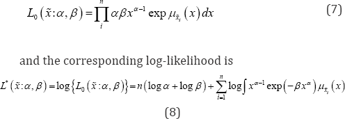
Since the data vector X is a realization of a random vector X drawn independent identically distributed and assuming the decomposable joint membership function u (x) as in Eq. (6) the likelihood function can be presented as
Parameter estimation of a distribution
The theory of parameter estimation is huge and there are many methods available to estimate parameters of a particular distribution. In common practice, the methods which are used in parameter estimation of a distribution include
Method of moments
Let X = (X1,,X2....xn) be independent and identically distributed (iid) random variables with a probability density function f (x ;θi,θ2,....θn), where (θ1,θ2,....θn) are the unknown population parameters. One of the oldest and simplest methods for finding estimators for one or more population parameter is the method of moments. Let μk=E(xk) is the kth moment measured from origin of a random variable X , provided it exists. Further let  bethe moments obtained from corresponding, then bythe method of moments estimator of μk is given by mk.
Method of least square
Method of least square (LS) is a popular choice in estimation theory. In general LS method estimates the parameter by minimizing the error function. But there are other forms of LS too such as Least Root Mean Square, Least Median Square.
Method of maximum likelihood estimation (MLE)
MLE is a method of parameter estimation very frequently used in statistics and is a crucial tool for many statistical modeling procedures [19]. Let X = ( x1,, X2....xn) be a random sample drawn independently and identically (iid) from a probability density function f(x;θ1θ2.....θn ) where (θ1θ2.....θn ) are the unknown population parameters and  is the log-likelihood function, then l— log [rif(x;e,e. e)J is the log-likelihood function. MLE's can be obtained by maximizing the log likelihood function with respect to the desired parameters. But in many cases close functional forms of the estimators may not be obtained, in that case the procedure that generally adopted are iterative in nature which includes in general numerical methods like Newton
Raphson's method, very well known method which is used in most of the cases is Expectation maximization algorithm (EM). Bayesian method is another approach of parameter estimation and some of these methods will be discussed in the following section.
MLE of parameters of weibull distribution when nature of the data is not precise
Method of maximum likelihood estimation maximizes the likelihood function with respect to the parameter. Maximum likelihood method is most commonly used method in parameter estimation and is considered as most robust, which yield estimators with good statistical properties. The MLE for the pdf in Eq. (1) i.e. the parameters a and p can be obtained by partially differentiating log-likelihood function (8) with respect to the parameters and then equating to zero. The partial derivative of (8) with respect to α and β are:
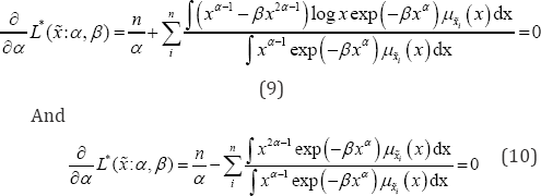
From the above expressions (9, 10) it can be observed that there are no closed forms for the solution are possible, an iterative approach can be useful to find the solution for and In the subsequent section, we are going to discuss some of the p methods applied to obtain the solution of the parameters.
Graphical approach
In this approach, we are mainly looking to get a solution by the help of plots. Form equation (10) λ can be written as:

Let us denote R.H.S of (11) as H(x:a,p); if h(x:a,p) is strictly increasing with increasing values of p it can be expected that 1 p and h(x:a, p) will intersect exactly at one point since 1/p is strictly decreasing as β→∞
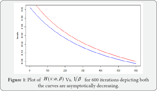
Note: Graphical approach to finding MLE as suggested by Balakrishnan & Kateri [2] does not give us a promising result as depicted by the above plot (Figure 1).
EM algorithm
The Expectation-Maximization (EM) algorithm is a broadly applied method to obtain the maximum likelihood estimators iteratively. An iteration of the EM algorithm consists of two steps- called the Expectation step or the E-step and the Maximization step or the M-step. From equation (4) log likelihood function corresponding to the complete data x becomes

Partial derivative of Eq. (12) with respect to a , fi gives the following equations

EM algorithm is presented by the below iterative steps Given the initial values of α and β say α(0) and β(0) at In the (h+1)th step of the algorithm,
The first step of the algorithm i.e. Expectation step is presented by the computation of conditional expectations as below
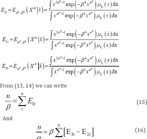
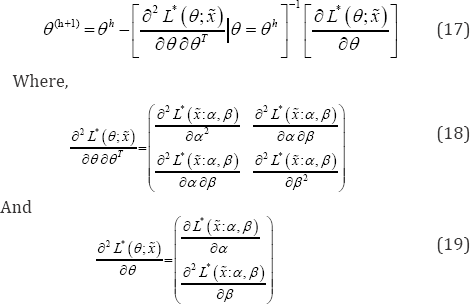
The M-step requires solving equations (18) and (19) and obtaining the values of (α(h+1), β(h+1)).
NR algorithm
NR algorithm is another iterative method to find MLE. Let θ=(α,β)T be the desired parameter to be estimated. Then, at (h+1)th iteration the estimates of the parameters are given by
Bayesian estimation
While we have discussed about the use of the EM algorithm for finding MLEs in a frequentist framework, EM algorithm can also be equally applied to find the nature of the posterior distribution under a Bayesian framework. Suppose n(0) is the distribution of prior for the parameters θ=(α,β)T then,

is the likelihood function of posterior distribution of the parameters. The expectation step is in fact the same as for the frequentist framework where computation of the MLE of d=(a,p)T is carried out by conditional expectation of the complete-data log likelihood.
Let us consider θ=(α,β)T has priors according as α~G(c,d), β~G(a,b), then the likelihood function based on is

Then, considering the loss function as squared error loss function, estimate of any function of 9=(a,P)T say g(O) under the Bayesian framework is

It is to be noted that equation (22) can't be solved analytically to obtain the expectation. Tierney & Joseph's [19] approximation procedure has been adopted for computation of Bayes estimate
for θ=(α,β)T
Neural network
Neural network is an iterative process in which we try to optimize the target output by minimizing error. The literature of neural network is vast and has been used for the parameter estimation of distributions by Wachowiak et al. [16] and Abbasi et al. [13]. In the present study, feed-forward neural network has been applied to estimate the parameters of Weibull distribution. An important aspect of neural network is determining its network architecture i.e. to determine the number of hidden layers units to each layer to be used. Teoh et al. [20] used singular value decomposition and presented the impact of increasing the number of neurons in the hidden layer of feed forward neural network architecture. The point of using neural network in parameters of Weibull distribution is that neural network can easily learn the input-output relationship without having any prior knowledge of the functional relationship between input and output [21].
The rth order moment for the probability density function presented in Eq. (1) is given by

Where Г(.) represents gamma function.
Form weak law of large numbers it is known that,

Where 'P' denotes convergence in probability. Thus, if we are concerned about getting the estimates of population moments, the method of moments provides consistent and unbiased estimators. By equating sample moments with that of population moments we get the below equations

Solving Eq. (25) and Eq. (26) estimates of the parameters α and β can be obtained. Since closed forms of solution cannot be obtained, artificial neural network (ANN) has been used to estimate α and β. Eq. (25), Eq. (26) shows that α and β are related to first and second order moments and hence sample moments are used as input to train the network. It is very much important to decide network architecture which involves the determination of the number hidden layer to be used and nodes in each of the hidden layers. Determination of the network architecture depends on the complexity of the problem at hand. An ideal network corresponding to input output data set is determined experimentally based on the RMSE. Moreover, the objective of training neural networks is not limited to learn an exact depiction of the training data, rather to build a model based on the training set which can generalize the new input data set that we usually call test data. In practice if the feed forward neural network is over-fit to the noise on the training data, it memorizes the training data and gives poor generalization to a test data set. The network architecture used in the present study is not fixed, based on the sample at hand different network structure has been used for training. Matlab Math Works and R 3.0.3 are used for the analysis purpose. The generated data is randomly divided into three parts namely training, testing and validation set. The percentages of data being used are 50, 30, and 20. The problem of over fitting is avoided by analyzing the neural network performance after training [22,23]. Data generation and analysis
Simulation allows us to compare different analytical techniques. Monte Carlo simulation has been used to simulate data of different sample sizes for Weibull random variable and are then fuzzyfied using the following membership functions.
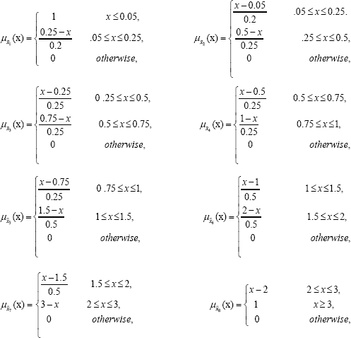


The average values and mean squared errors (MSE) of the estimates over 1000 replications are presented in Table 1 and Table 2
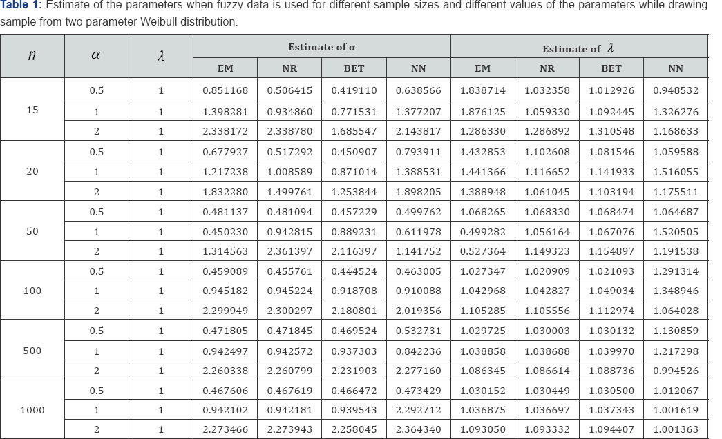
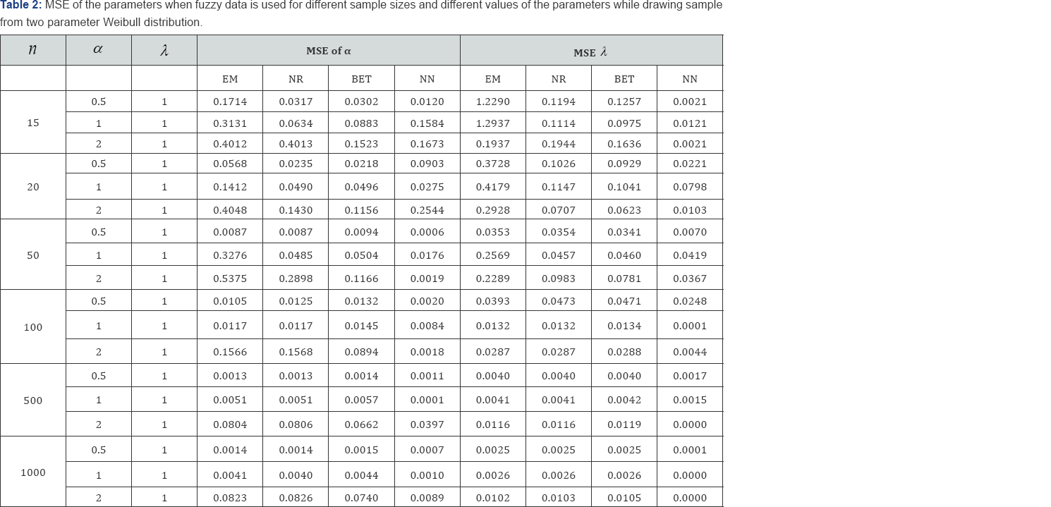
The estimates for the parameters and are computed using fuzzy data. Estimation method includes maximum likelihood method (via NR and EM algorithms), artificial neural network (ANN) and a Bayesian procedure. For computing the Bayes estimates information about the prior distribution of the parameters is needed. It is assumed that and follow Gamma (a, b) and Gamma (c, d) priors respectively. To carry out the comparison it is further assumed that the priors distribution of the parameters are non-informative, and a = b = c = d = 0. The performance of the ANN network structure used for the analysis. Since in this study different sizes have been used, we did not limit ourselves to particular network architecture. The type of network used is Feed-forward backpropagation neural network and the number of hidden units is determined using Teoh et. al. (2006) Inputs to the network were the 1st and 2nd order moments of the generated samples; randomly selected 20% of the samples were used in testing.
Conclusion
Based on complete and censored data some work on Parameter estimation of Weibull distribution has been done previously. But, generally it is assumed that the data at hand are exact numbers. However, it may happen that some of the collected data are imprecise and are represented in the form of fuzzy numbers. Therefore, we need suitable methodology to handle these data as well. This paper shows that the traditional methods usually used in parameter estimation based on methods of moments or maximum likelihood function did not come out with the explicit solution, when nature of the data is considered as fuzzy. Instead iterative methods were used to estimate the parameters. Iterative methods used involve complex calculation and its computation is tedious. The proposed approach based on neural network to estimate parameters of Weibull distribution showed a significant improvement. It has been found that apart from the small samples neural network performance was better compared to the other methods. The main advantage of using neural network is that neural network does not require complex theoretical derivations and tedious computations as well.
Ethics
This is not applicable since the submitted paper is not related to field work, only based on mathematical assumptions in the field of Inferential Statistics.
Data accessibility
We have written our manuscript in the field of statistics and also done comparisons along with other existing schemes which are given in references. Thus, there is no need for data accessibility.
Authors contribution
Both authors (Gajendra K. Vishwakarma, Chinmoy Paul and Neha Singh) have equal contributions to this manuscript.
Funding
There is no funding because Chinmoy Paul (As a second author) and Neha Singh (As a third author) are doing PhD as a full-time research scholar under the supervision of Gajendra K. Vishwakarma (As a first author) from Department of Applied Mathematics, Indian Institute of Technology Dhanbad, India-826004.
Funding
We thank our Institute i.e., Indian Institute of Technology Dhanbad, India-826004 in which Chinmoy Paul and Neha Singh are doing PhD as full-time research scholar and Dr Gajendra K. Vishwakarma is working as an Assistant Professor in the Department of Applied Mathematics.
References
- Smith TF, Waterman MS, Sadler JR (1983) Statistical characterization of nucleic acid sequence functional domains. Nucleic acids research 11(7): 2205-2220.
- Hawley DK, McClure WR (1983) Compilation and analysis of Escherichia coli promoter DNA sequences. Nucleic acids Res 11(8): 2237-2255.
- Schneider TD, Stormo GD, Gold L, Ehrenfeucht A (1986) Information content of binding sites on nucleotide sequences. J Mol Biol 188(3): 415-431.
- Schneider TD, Stephens RM (1990) Sequence logos: a new way to display consensus sequences. Nucleic acids Res 18(20): 6097-6100.
- Bembom O (2017) seqLogo: Sequence logos for DNA sequence alignments. R package version 1.44.0.
- Crooks GE, Hon G, Chandonia JM, Brenner SE (2004) WebLogo: a sequence logo generator. Genome Res 14(6): 1188-1190.
- Wagih O (2014) RWebLogo: plotting custom sequence logos. R package version 1.0.3.
- Thomsen MCF, Nielsen M (2012) Seq2Logo: a method for construction and visualization of amino acid binding motifs and sequence profiles including sequence weighting, pseudo counts and two-sided representation of amino acid enrichment and depletion. Nucleic Acids Res 40(W1): W281-W287.
- Wu X, Bartel DP (2017) kpLogo: positional k-mer analysis reveals hidden specificity in biological sequences. Nucleic Acids Res 45(W1): W534-W538.
- Ou J, Stukalov A, Nirala N, Acharya U, Zhu LJ (2018) dagLogo: dagLogo. R package version 1.16.1.
- O'shea JP, Chou MF, Quader SA, Ryan JK, Church GM, et al. (2013) pLogo: a probabilistic approach to visualizing sequence motifs. Nat Methods 10(12): 1211-1212.
- Colaert N, Helsens K, Martens L, Vandekerckhove J, Gevaert K (2009) Improved visualization of protein consensus sequences by iceLogo. Nature Methods 6(11): 786-787.
- Dey KK, Xie D, Stephens M (2017) A new sequence logo plot to highlight enrichment and depletion. bioRxiv P.226597.
- Wagih O (2017) ggseqlogo: a versatile R package for drawing sequence logos. Bioinformatics 33(22): 3645-3647.
- Hofmann H, Hare E, GGobi Foundation (2017) gglogo: Geom for Logo Sequence Plots. R package version.
- Ou J, Wolfe SA, Brodsky MH, Zhu LJ (2018) motifStack for the analysis of transcription factor binding site evolution. Nature Methods 15(1): 8-9.
- Mahony S, Benos PV (2007) STAMP: a web tool for exploring DNA- binding motif similarities. Nucleic Acids Res 35(suppl_2): W253-W258.
- Nettling M, Treutler H, Grau J, Keilwagen J, Posch S, et al. (2015) DiffLogo: a comparative visualization of sequence motifs. BMC bioinformatics 16(1): 387.
- Vacic V, Iakoucheva LM, Radivojac P (2006) Two Sample Logo: a graphical representation of the differences between two sets of sequence alignments. Bioinformatics 22(12): 1536-1537.
- Kopp W, Vingron M (2017) An improved compound Poisson model for the number of motif hits in DNA sequences. Bioinformatics 33(24): 3929-3937.
- Sandelin A, Alkema W, Engstrom P, Wasserman WW, Lenhard B (2004) JASPAR: an open-access database for eukaryotic transcription factor binding profiles. Nucleic Acids Res 32(suppl_1): D91-D94.
- Kheradpour P, Kellis M (2013) Systematic discovery and characterization of regulatory motifs in ENCODE TF binding experiments. Nucleic Acids Res 42(5): 2976-2987.
- Kulakovskiy IV, Medvedeva YA, Schaefer U, Kasianov AS, Vorontsov IE, et al. (2012) HOCOMOCO: a comprehensive collection of human transcription factor binding sites models. Nucleic Acids Res 41(D1): D195-D202.
- Kulakovskiy IV, Vorontsov IE, Yevshin IS, Soboleva AV, Kasianov AS, et al. (2015) HOCOMOCO: expansion and enhancement of the collection of transcription factor binding sites models. Nucleic acids research 44(D1): D116-D125.
- Kulakovskiy IV, Vorontsov IE, Yevshin IS, Sharipov RN, Fedorova AD, et al. (2017) HOCOMOCO: towards a complete collection of transcription factor binding models for human and mouse via large-scale ChIP-Seq analysis. Nucleic Acids Res 46(D1): D252-D259.
- Koch CM, Andrews RM, Flicek P, Dillon SC, Karaoz U, et al. (2007) The landscape of histone modifications across 1% of the human genome in five human cell lines. Genome Res 17(6): 691-707.
- Alexandrov LB, Nik-Zainal S, Wedge DC, Aparicio SA, Behjati S, et al. (2013) Signatures of mutational processes in human cancer. Nature 500(7463): 415-421.


