


Biplots in Covariance Analysis
Opeoluwa FO1* and Sugnet L2
1Department of Statistics and Population Studies, University of Namibia, South Africa
2Department of Statistics and Actuarial Science, Stellenbosch University, South Africa
Submission: September 12, 2017; Published: November 10, 2017
*Corresponding author: Opeoluwa F Oyedele, Department of Statistics and Population Studies, University of Namibia, South Africa, Fax: +264612063791,Tel: +264612064515; Email: OpeoluwaOyedele@gmail.com
How to cite this article: Opeoluwa F, Sugnet L. Biplots in Covariance Analysis. Biostat Biometrics Open Acc J. 2017;3(4): 555623. DOI: 10.19080/BBOAJ.2017.03.555623
Abstract
Among the various statistical techniques useful for exploring the relationships between different sets of variables is the Covariance Analysis. Since biplots in general are useful graphical tools for exploring the relationships between (multivariate) variables, the biplot is employed in the covariance analysis framework to form the covariance biplot. The resulting biplot provides a single graphical display of the variables and inter-variables relationships. An illustration is shown using a mineral sorting production data consisting of five hundred and seventy-two processes.
Keywords: Biplots; Covariance matrix; Monoplots; Variance-covariance matrix
Abbreviations: PCA: Principal Component Analysis; CA: Correspondence Analysis; MCA: Multiple Correspondence Analysis; CVA: Canonical Variate Analysis; MDS: Multi-Dimensional Scaling; DA: Discriminant Analysis; GLMs: Generalized Linear Models; PLS: Partial Least Squares
Introduction
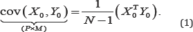
In a situation where the relationships between different sets of variables are of interest, various statistical techniques can be useful tools for analysis. Among them is the covariance matrix.Consider two centered matrices X0:N x P and Y0:Nx M The covariance between x0 and Y0 is defined by
However, when only one set of variables is under consideration, the variance-covariance matrix is defined by
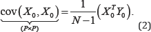
This is also written as cov(X0,X0)=var (X0,X0)=cov(X0)Here, the variances of X0 are given in the diagonal of (2), while the covariances are shown off-diagonal. The relationships between different sets of variables can be explored using some form of graphical display such as biplots [1,2]. Since biplots are useful graphical tools for exploring the relationships between variables, the biplot is employed in the form of the covariance biplot. In this paper, the general idea behind the covariance biplot is discussed. It further demonstrates, with graphical illustrations, how the covariance biplot can help to reveal variables and inter-variables relationships. This paper is a progressed work of Oyedele & Gardner-Lubbe [3].
The remainder of this paper is organized as follows. Section 2 provides a brief overview of the biplot and its fundamental idea, before its employment in the form of the covariance biplot is discussed in Section 3. This is followed by an application with a mineral sorting production data that shows the quality evaluation of five hundred and seventy-two processes used to produce a final product in Section 4. Finally, some concluding remarks are offered in Section 5.
Biplots
Time and again, biplots, to be precise, asymmetric biplots, are often referred to as the multivariate version of scatter plots. In the usual two-dimensional scatter plot, two orthogonal Cartesian axes are used for reading off the values of the sample points, as well as for adding points to the plot. The fact that biplots are referred to as multivariate scatter plots implies that more than two variables are represented by (non-orthogonal) axes [4,1]. Just like scatter plots, biplots are helpful for revealing clustering, multivariate outliers, variables and inter-variable relationships of a data set [2]. An advantage of the biplot is that it allows for the visual assessment of a high-dimensional data matrix in a two- or three-dimensional plot.
Since the biplot was first introduced by Gabriel [5], its theory has been significantly extended with Gower & Hand's [1] monograph, Yan & Kang's [6] description of various methods to visualize and interpret a biplot, Greenacre’s [7] text on the use of biplots in practice and Gower, Lubbe and Le Roux's [8] illustration of the construction of various forms of biplots. In the first biplots introduced by Gabriel, the rows and columns of a data matrix were represented by vectors, but to differentiate between these two sets of vectors, Gabriel [5] suggested that the rows of the data matrix be represented by points. Gower & Hand [1] went a step further by introducing the idea of representing the columns of the data matrix by axes, rather than vectors, while still representing the rows of the data matrix by points. This was done to support their theory that biplots were the multivariate version of scatter plots. Gower & Hand's [1] biplot representation is very useful when the data matrix under consideration is a matrix of samples by variables.

An example of the biplot display of the chemical-sensory data by Mevik & Wehrens [9] is shown in Figure 1. This data shows the sensory descriptors and the chemical quality measurements of sixteen olive oils. In this biplot display, a representation of the variance of each variable is provided. This is represented by the thicker arrow (vector) on each axis in each display. For example, the standard deviation of Acidity is smaller compared to the others, while DK has a large deviation. This is evident from the length of the vector on these axes. Furthermore, several relationships can be deduced from this biplot, such as a relation between Syrup, K232 and Peroxide. Another relationships deduction is the relation between K270, Transp and Glossy, and between Green, Yellow and DK. These relationship deductions are done based on the angle between axes.
Since 1971, biplots have been employed in a number of multivariate methods as a form of graphical representation of data, pattern and data inspection, as well as for displaying results found by well-known statistical methods of analysis [1012]. The most well-known methods are Principal Component Analysis (PCA), Correspondence Analysis (CA), Multiple Correspondence Analysis (MCA), Canonical Variate Analysis (CVA), Multi-Dimensional Scaling (MDS), Discriminant Analysis (DA), Generalized Linear Models (GLMs), and recently, Partial Least Squares (PLS) by Oyedele & Lubbe [13]. All these forms of biplots have been applied to diverse fields of specialization, according to different needs and requirements.
Fundamental idea of biplots
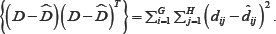
A biplot is a joint graphical display of the rows and columns of a data matrix D (of G rows and H columns) by means of markers a1,a2,.....,aG for its rows and markers b1,b2,.....,bH for its columns. Each marker is chosen in such a way that the inner product aiTbj represents di,j, the (i,j)th element of the data matrix D [14]. Biplots are often constructed in two dimensions. This does not mean that they are limited to two dimensions, but this is the most convenient biplot display. However, with D being a (very) large matrix, the rank of D is almost always higher than two. As a result, some approximation is done on D to obtain a lower rank. Methods such as PCA can be used to perform this approximation. In PCA, the approximation is based on the method of least squares. To be precise, the sum-of-squares of the differences between D and its approximation  is minimized. That is, minimize trace
Taking as the rank two approximation of D, the biplot of a data matrix D relies on the decomposition of into the product of two matrices,

its row markers matrix (A) and its column markers matrix (B). Matrices A and B are defined as
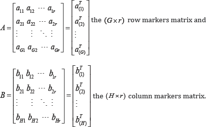
Thus, the approximated rows and columns of a data matrix are represented in biplots. Generally, the number of columns in A and B are determined by the rank r approximation of D. In practice, r=2 is usually preferred for a convenient biplot display.
Biplot points and axes
In asymmetric biplots, the rows of a data matrix are represented by points, while the columns are represented by vectors or axes. Traditionally, columns are represented by vectors, but Gower & Hand [1] introduced axes to make the biplot similar to a scatter plot. This was done by extending the vectors, which represent the columns, through the biplot space to become axes. Thus, the biplot points will be defined by the row markers of the data matrix, whereas the biplot axes will be defined by the column markers. More precisely, for the biplot of a data matrix D, from equation (3), G rows of A will serve as the biplot points, while H rows of B will be used in calculating the directions of the biplot axes. An example of the biplot display can be seen in Figure 2.

Biplot implementation into covariance analysis framework

In general, there are two kinds of features displayed in biplots. These features can be specified as two sets of variables, or as a set of variables and samples, as in the case of the PCA biplot. This does not mean that biplots cannot be constructed by using only one kind of feature, but depending on the data matrix and the choice of features to be analyzed, biplots can be constructed to display only one kind of feature. Gower, Lubbe and Le Roux [8] termed such biplots monoplots. In a monoplot, the kind of feature to be represented may be the samples only or one set of variables. Including an additional feature in the monoplot, say, another set of variables, would result in a biplot. As only variables are represented in the covariance and variance-covariance matrices, see equations (1) and (2), both monoplots and biplots can be used as graphical tools to explore their relationships. More precisely, a monoplot would be suitable for representing a variance-covariance matrix (equation (2)) graphically, while a biplot would be more appropriate for a covariance matrix (equation (1)). An example of the resulting monoplot display can be seen in Figures 3 & 4, while an example of the resulting biplot display can be seen in Figure 2.

Covariance monoplot
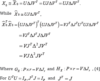
Consider the X-variables only. By the Singular Value Decomposition(SVD),X0=UΔVT,for U : N×P,Δ:P×P and V : P×P Defining the matrices 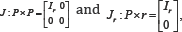 it follows that
Since GX = Hx in (4), the rows of either GX or Hx will be used in the monoplot.
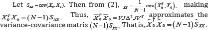
Moreover, given that only one set of variables, in this case , is under consideration, and as the focus is on revealing the relationships within these variables, only one set of axes is needed. From expression (4), the directions of these axes are calculated by the P rows of either Gx or Hx .
Covariance biplots
Consider both x0 and Y0 The P×M covariance matrix between x0 and Y0 is defined in equation (1). Let Sxy= cov(x0,Y0).By the SVDSxy = DΛFT,, forD:P×M, Λ:M×M and F: M×M . The matrix SXY=DΛFT, can be written as
Sxy≌ Ŝxy= DΛJFT= DΛJΛFT= DJΛJFT= GHT
Where
G= DΛβJ, and H = FΛ1-βJ for any value of β ϵ (0,1) (5)
In expression (5), the matrix J has dimension M×M while the matrix Jr has dimension M×r The matrix G: P× r contains the information about the X-variables, while matrix H :M × r contains the information about the Y-variables.
Since,  the inner-product between the rows of the matrix G and the rows of the matrix H approximates the covariances between the X-variables and the Y-variables. Here, the rows of G associates with the X-variables, while the rows of H associates with the Y-variables. Focusing on revealing the relationships between two sets of variables, X and Y, only axes will be present in the resulting biplot. However, two sets of axes are needed, a set for the X-variables and a set for the Y-variables. the directions of the axes representing the X-variables are calculated using the P rows of G, while M rows of H are used to calculate the directions of the axes representing the Y-variables. This biplot, called the covariance biplot, reveals the relationships between the two sets of variables as well as within each set.
From expression (5), when β = 1,
G = DΛ1Jr = DΛJr and H = FΛ1-1 Jr = FJr.
Also,
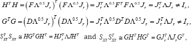
HTH = (FJr )T (FJr )= JTrFTFJr = JrTJr = Ir
And
GTG = (DΛJr)T(DΛJr)= JTrΛDTDΛJr= JTrΛ2Jr ≠ Ir
Where
FTF = IM, JTrJr = Ir and DTD =IM For this choice of ,
SXYSTXY≅ GHT HGT = GGT
But
SXYSTXY≅ HGTGHT = HHT .
Therefore, from SXYSTXY≅ GHT the row markers G approximate the covariance between the rows of SXY the rows of SXYare associated with the X-variables, the rows of G approximate the covariance between these X-variables.
Conversely, whenβ = 0 ,
G = DΛ0 Jr = DJr and H = F Λ1-0 Jr = FΛJr.
GTG = (DJr)T (DJr) = JTrDTDJr = JTrIr = Ir Now,
For DTD = IM and JTrJr = Ir, but
HTH = (FΛJr)T (FΛJr) = JTrΛFTFΛJr = JTr Λ2Jr ≠ Ir
Where FTF = IM. Thus,
STXYSXY ≅ HGTGHT = HHT
And
SXYTSXY ≅GHTHGT≠GGT.
From SXYTSXY≅HHT, the column markers H approximate the covariance between the columns of SXY. In other words, with the columns of SXY associated with the Y-variables, the rows of H approximate the covariance between these Y-variables.
Moreover, any β value between 0 and 1 will neither optimally approximate the covariance between the X-variables nor the covariance between the Y-variables, but rather, it will give an indication of both. Since choosing β closer to 0 better approximates the covariance between the Y-variables, the symmetric choice of  will be used in the biplot.
With the choice of β = 0.5, covariance between the X- and Y-variables is both equally approximated, although not optimal for either. That is, for G= DΛ05Jr H = FΛ1-0.5Jr = FΛ0.5Jr,
Where FTF=IM and DTD = IM . In this situation, the rows of HJTrΛ0.5. approximate (non-optimally) the covariance between the Y-variables, while the rows of GJRrΛ05 approximate (non- optimally) the covariance between the X-variables. In line with equation (1), the approximated covariance can be written as
Thus, in expression (5), β = 0 only caters for the covariance between the Y-variables optimally, while β = 1 only caters for the X-variables optimally. On the other hand, β = 0.5 caters for both X- and Y-variables equally, although not as optimally as when only one set is been catered for.
It should be noted that since only variables are being represented in the covariance monoplot/biplot and there are no samples to (orthogonally) project onto the axes representing these variables, calibration markers are not necessary on these axes.
An Illustration
The following illustration of the covariance biplot is performed using the SOVR data from Umetrics MKS [15]. This mineral sorting production data shows the quality evaluation of five hundred and seventy two processes used to produce a final product. Twelve process factors were used in the evaluation, namely, total load (TON_IN), load of grinder 30 (KR30_IN), load of grinder 40 (KR40_IN), concentration mull (PARM), velocity of separator 1 (HS_1), velocity of separator 2 (HS_2), effect of grinder 30 (PKR_30), effect of grinder 40 (PKR_40), ore waste (GBA), load of separator 3 (TON_S3), waste from grinding (KRAV_F) and total waste (TOTAVF). The aim of this evaluation was to investigate the relationships between the process factors and the quality of the final product. Six output variables, amount of concentration type 1 (PAR), amount of concentration type 2 (FAR), distribution of concentration type 1 and 2 (r-FAR), iron in FAR (Percent_Fe_FAR), phosphor in FAR (Percent_P_FAR) and iron in raw ore (Percent_Fe_malm), were used to measure the quality of the final product. The processes are assigned as the samples, while the process factors and output variables are the predictor and response variables respectively. Thus, the SOVR data can be viewed as a 572x18 data matrix, comprising of an X:572x12 matrix and a Y:572x6 matrix. A copy of this data can be found on the dropbox link [reference] under the "Data Sets" folder [16].
As is customary for covariance analysis, both the X:572×12 and Y:572 × 6 matrices are centred before the analysis. In addition, each of these matrices is standardized by dividing each centred variable by their respectively standard deviation, as this facilitates the direct comparison of correlation values. The (twodimensional) covariance biplot for the data is shown in Figure 2, with β = 0.5. The respective G:5×2 and H:6×2 matrices are shown in Tables 1 & 2 respectively. The approximated covariance values are shown in Table 3. The representation of the variance of each variable, represented by the thicker arrow (vector) on each axis, is shown in the biplot displays (Figures 2 to 4). Observing the length of the thicker arrows (vectors) on the axes in Figure 1, output variables PAR and FAR can be said to have the largest standard deviation. However, variable Percent_ Fe_malm has the smallest standard deviation, compared to the others, followed by process factor HS _1. These deductions can also be seen (clearly) in Figures 3 & 4.


Furthermore, the positions of the biplot axes give an indication ofthe correlations between the variables. Axes forming small angles are said to be strongly correlated - either positively or negatively. Axes are positively correlated when they lie in the same direction, while negatively correlated axes lie in opposite directions. Also, axes that are close to forming right angles are said to be uncorrelated. From Figure 2, various inter-variable relationships can be deduced, such as the relation between output variables FAR and r_FAR and process factors TOTAVF,GBA, PKR_40, KR30_IN, TON_IN, KR40_IN, KRAV_F and PKR_30. Looking at the directions of these axes in the biplot, this relation is a positive one. Also, the relation between process factor HS_2 and output variables Percent _ P _ FAR and Percent_Fe _FAR can be seen. The relation between factor HS_2 and Percent _ P _ FAR is a negative one, while the relation between factor HS_2 and Percent _Fe _FAR is a positive one. However, process factor Percent_Fe_maltn can be said to have no relation with the others.


Moreover, to illustrate how a covariance monoplot can help to reveal relationships within one set of variables, consider the monoplot of the process factors shown in Figure 3. From this monoplot display several relationships can be deduced, such as the relation within process factors TOTAVF, GBA, PKR_30, KRAV_F, TON_IN, KR40_IN, KR30_IN and PKR_40, with an approximated (positive) correlation values of 0.944, 0.876, 0.907, 0.927, 0.918, 0.900 and 0.921 respectively as shown in Table 4. Factors TON_ S3, HS_1 and HS_2 can be said to be unrelated to each other. Likewise, from the covariance monoplot of the output variables (Figure 4), output variables r_ FAR , PAR and FAR can be said to be related, with an approximated (positive) correlation values of 0.675, 0.705 and 0.920 respectively as shown in Table 5. Also, a (negative) relation within variables Percent_P_FAR and Percent _Fe _FAR (-0.864) can be noted.
Conclusion
The covariance matrix of two sets of variables can be visualized graphically using the biplot. The resulting biplot, termed the covariance biplot, reveals variables relationships graphically. If only one set of variables is considered in the covariance analysis, the resulting graphical representation is a covariance monoplot. Advantages of a covariance biplot include the revelation of the relationships between two sets of variables as well as within each set.
Software
The SOVR data can be obtained from the dropbox link [16] under the "Data Sets" folder. A collection of functions has been developed in the R programming language [17] to produce the biplot display of the chemical-sensory data in Figure 1 and the covariance biplot and monoplot displays of the SOVR data in Figures 2-4. These functions are available in the R package called PLSbiplot1 by Oyedele [18], and can be found on the Comprehensive R Archive Network (CRAN)'s repository, at [19] A detailed documentation for all the routines in this package can be found on the dropbox link, [20]
The following R code were used to obtain Figures 1-4
# Install the PLSbiplot1 package
# First download the PLSbiplot1_0.1.tar.gzfile from the
# CRAN at [19] and install into R.
#Load the PLSbiplot1 package require (PLSbiplot1)
#Olive oil data
if(require(pls))
data(oliveoil, package="pls")
Dmat = as.matrix(oliveoil)
dimnames(Dmat) = list(paste(c("G1","G2","G3","G4","G5","I1","I2","I3","I4","I5","S1","S2","S3","S4","S5","S6")),
paste(c('Acidity","Peroxide","K232","K270",”
DK","Yellow","Green","Brown","Glossy","
Transp","Syrup")))
#The biplot display
PCA.biplot(D=Dmat, method=mod.PCA, ax.tickvec. D=c(8,5,5,7,6,4,5,5,8,7,7))
#Here, the data was approximated using PCA to obtain a
lower rank of 2
#Refer to Section 2.1 above.
SOVR data
SOVR_data = read.table(file.choose(), header=TRUE)
#X-variables
X = as.matrix(SOVR_data[,1:12],
ncol=12)
#Y-variables
Y = as.matrix(SOVR_data[,13:18], ncol=6)
# The covariance biplot displays
cov.biplot(X,Y) #for both X- and Y-variables
cov.biplot(X,X) #for X-variables
cov.biplot(Y,Y) #for Y-variables
Acknowledgement
Professor Sugnet Lubbe is thanked for her valuable contributions.
Conflict of Interest
There are no economic interests and no conflict of interests.
References
- Gower JC, Hand DJ (1996) Biplots. Chapman & Hall: London, UK.
- Kohler U, Luniak M (2005) Data Inspection using Biplots. The Stata Journal 5(2): 208-223.
- Oyedele OF, Gardner L, Sugnet (2014) The Covariance Biplot to Reveal Relationships between Different Sets of Variables. Int Sci Technol J Namibia 3(1): 107-113.
- Gardner L, Le R, Maunders H, Shah V, Patwardhan S (2009) Biplots for Exploratory Analysis of Gene Expression Data. Statistical Analysis and Data Mining 2: 135-145.
- Gabriel KR (1971) The Biplot Graphic Display of Matrices with Application to Principal Component Analysis. Biometrika 58(3): 453467.
- Yan W, Kang MS (2003) GGE Biplot Analysis. CRC Press: Boca Raton, FL, USA.
- Greenacre MJ (2010) Biplots in Practice. Fundacion BBVA: Barcelona, Spain.
- Gower JC, Lubbe S, Le Roux (2011) Understanding Biplots. John Wiley & Sons: Chicester, UK.
- Mevik BH, Wehrens R (2007) The pls Package: Principal Component and Partial Least Squares Regression in R. Journal of Statistical Software 2(18): 1-24.
- Bradu D, Gabriel KR (1978) The Biplot as a Diagnostic Tool for Models of Two-Way Tables. Technometrics 20(1): 47-68.
- Constantine AG, Gower JC (1978) Graphical Representation of Asymmetry Matrices. Journal of the Royal Statistical Society 27(3): 297-304.
- Gabriel KR (1981) Biplot Display of Multivariate Matrices for Inspection of Data and Diagnosis. In Barnett V (ed.), Interpreting Multivariate Data, Wiley: Chicester, UK, pp. 147-173.
- Oyedele OF, Lubbe S (2015) The Construction of a Partial Least Squares Biplot. Journal of Applied Statistics 42(11): 2449-2460.
- Barnett V (1981) Interpreting Multivariate Data. Wiley Series in Probability and Mathematical Statistics. Wiley: New York, USA.
- Umetrics MKS (2013) SIMCA-P+. Version 12.
- https ://www. dropbox.com/sh/wr6 6u0 7t1vjm9 da/AACg_ E4h8MvgOHuCXk69yDIya
- R Core Team (2014) R: A Language and Environment for Statistical Computing. Foundation for Statistical Computing, Vienna, Austria.
- Oyedele OF (2014) The Construction of a Partial Least Squares Biplot.University of Cape Town, South Africa.
- https://cran.r-project.org/


