


A Note on Transition Models for Binary 2 x 2 Cross-Over Data
Takuma K1, Asanao S2 and Etsuo M2
1Department of Applied Mathematics, Tokyo University of Science, Japan
2Department of Mathematics, Tokyo University of Science, Japan
Submission: September 22, 2017; Published: October 27, 2017
*Corresponding author: Takuma Kurosawa, Department of Applied Mathematics, Graduate School of Science, Tokyo University of Science, Japan, Tel: +8190-5329-6165; Email: t.kurosawa1106@gmail.com
How to cite this article: Takuma K, Asanao S, Etsuo M. A Note on Transition ransition Models for Binary 2�2 Cross-Over Data. Biostat Biometrics Open Acc J. 2017;3(5): 555622. DOI: 10.19080/BBOAJ.2017.03.555622
Abstract
This paper presents a transition model within the framework of a generalized linear model for binary cross-over data. As a simple example, an analysis of binary 2 x 2 cross-over data on cerebrovascular deficiency is used to illustrate the model. Several simulation studies are carried out to assess the asymptotic properties of the estimators of the parameters included in the model, with finite sample size, and to compare common methods with respect to the hypothesis test corresponding to the treatment effect. As a main result, we show that the estimators' asymptotic properties work with a moderate sample size, and the transition model takes the highest value with respect to the empirical power among the compared methods.
Keywords: Binary data analysis; Cross-over trial design; Generalized linear model; Partial likelihood
Introduction
The parallel-groups trial design has been studied for decades and is widely used, particularly in medicine and the health sciences. In this design, each unit is randomized to receive a treatment. On the other hand, in a cross-over trial design, each unit receives a sequence of treatments. A cross-over trial design is distinguished from a parallel-groups trial design, although the aim is typically to compare the effects of individual treatments. There are many possible sets of the sequences in a crossover trial design. The simplest one, called 2 x 2 design, has two treatments and two periods. In such a design, half the units in the trial receive treatment A and then, after an appropriate period, receive treatment B. The remaining units receive treatment B first and then switch to treatment A. This feature has advantages and disadvantages. As shown in the above 2 x 2 design example, all units result in a direct comparison of the treatments, because each unit takes some treatments and has the same sample- specific effects. Nevertheless, the comparisons are affected by the sequence of treatments, even if all treatments are identical. Therefore, the main aim of the cross-over trial is to remove the factors related to the differences between the samples from the comparisons.
Various cross-over trial designs have been proposed to remove such factors. For normally distributed 2 x 2 cross-over data, using two-sample t-tests has been suggested by Chassan [1], and Hills & Armitage [2]. This technique is also applied to linear models for cross-over data. Jones and Kenward [3] give a good summary of these models. For non-normally distributed 2 x 2 cross-over data, the t-test can be replaced by nonparametric methods such as the Wilcoxon signed rank test or the Mann- Whitney U-test. These methods were described by Koch [4], Tudor & Koch [5], and Stokes et al. [6]. In the non-normal case, especially for binary cross-over data, Gart [7] applied the Mainland-Gart test to a logistic regression, and Altham [8] derived the same model from a Bayesian point of view. More recently, the test has been applied in various other fields [9,10].
However, these methods use procedures that assume a covariance structure, for example, in generalized estimating equations or generalized linear mixed models [11,12]. An exception to this is the generalized linear transition model used to analyze 2 x 2 binary cross-over data, as introduced by Miyaoka et al. [13]. In this study, we extend the method based on binary p-ordered transition models within the framework of a generalized linear model and compare it to existing methods used to analyze binary 2 x 2 cross-over data. Our method need not assume any covariance structures and can naturally incorporate past observations into the model.
Methods
Transition Model for Binary Observations
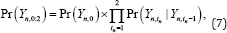
Let {Yn,tn} be a binary time series, where n = 1..,N and tn =‒p+1,---,Tn with arbitrary positive integer P . In addition, let {Zn,tn} be a covariate vector series that can include past observations. For samplen, if the primary event is observed at period tn then Yn,tn = 1 , otherwise, Yn,tn = 0 In keeping with standard practice, we refer to observations 1 and 0 as a success and a failure, respectively. For arbitrary t wo periods t1n < t2n let Yn,t1n:t2n be (Yn,t1n,...Yn,t2n) Using the simple decomposition rule, the joint probability of Yn,‒p+1:Tn is as follows:
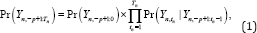
Under the assumption that the binary time series has the p-ordered Markov property, the joint probability can be rewritten as follows:
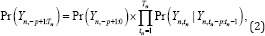
Let 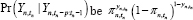 , which denotes a success or failure probability, given P observations that were observed in the previous periods.
We further suppose that
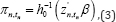
Where h‒10 is an appropriate inverse link function zn,tn and represents a transposition of zn,tn. If the joint probability Pr (Yn,‒p+1:0) in equation (2) is trivial or easy to find, we can use a full-likelihood estimation. However, in general, the joint probability is difficult to find. Thus, we eliminate the first term on the left-hand side of equation (2), and carry out the estimation based on a partial likelihood. The partial log-likelihood function is expressed as
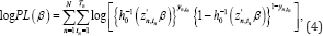
Then, the partial score function is given as
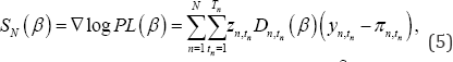
Where ▽ denotes a gradient, 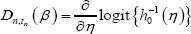 and η = z'n,tnβ the corresponding conditional information matrix is
Where 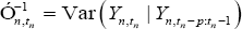 and Dn,tn(β) is the transposed matrix of Dn,tn(β). under normal regularity conditions, the maximum partial likelihood estimator
  is consistent and has asymptotic normality, with
 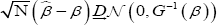 , where
 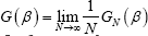 . The partial-Likelihood proposed by Cox [14], for conditional inference. Note that a more formal definition and theoretical validation for partial-likelihood was given by Wong [15] and Slud [16]. The partial-likelihood and maximum partial likelihood estimator for discrete-valued data are described in detail in Fokianos & Kedem [17,18]. The small sample behavior of this estimator is discussed in Kurosawa et al. [19].
Transition Model for Binary 2 x 2 cross-over data
For 2 x 2 binary cross-over data, let Tn = 2 and p=1 , equation (2) simplifies to
To calculate partial likelihood, we eliminate Pr(Yn,0) from equation (7) and assume that Yn,1 given (Yn,0) follows a Bernoulli distribution with parameter πn,1 = h‒11(Zn,1β) . For simplicity, let h0 and h1 are taken to be logit link functions. Then, the corresponding log-likelihood function is given as
Where h‒1 implies an inverse logit link function. Although there are various kinds of the covariate vector series {Zn,tn} we use the following parameterization as a simple example:


Where Zn,tn,1 is 1 if sample n received treatment A in period tnand 0 otherwise, and (Zn,tn,2 , Zn,tn,3) is (Yn,tn‒1,1‒Yn,tn‒1) if tn≥2 and otherwise both are 0. In this situation, parameter β1 denotes the treatment effect and the principle interest is to test the hypothesis H0 : β1 = 0 The parameters β2 and β3 represent a period effect and a test H0 : β2 = β3 indicates the absence of a period effect. Parameter β0 is the intercept. To illustrate the use of the transition model for 2 x 2 binary crossover data, we apply the data published by Jones & Kenward [3] to the model described above. Their original data were divided into two centers, however, in this example, we use data that were merged without considering differences in centers. The samples are randomized into two groups, namely group 1 and group 2. In group 1, each sample received treatment A at period 1 and treatment B at period 2. In group 2, each sample first received treatment B, and then treatment A. In Table 1, (i,j) denotes an ordered pair of two binary observations, where i and j represent the observation at period 1 and period 2, respectively.
The results are presented in Table 2. Focusing on β1 in the table, the effect of treatment A is likely to be positive. However, the Wald test statistic of 1.440 for the hypothesis β1 = 0 corresponding to a p-value of 0.075, leads us to conclude that there is insufficient evidence of a treatment effect. On the other hand, the likelihood ratio test statistic is 33.92 for the hypothesis β2 = β3 = 0, and the corresponding p-value is smaller than 0.001.

Results
Simulation results
We show two simulation results in this section. The first assesses the asymptotic properties of for a finite sample size, as described at transition model for binary observations, while the second compares the tendency to reject the principle interest hypothesis, which implies that the effects are different between treatments A and B. For all the simulations, we generated data 10,000 times for N = 40,60,80,100 and 200 samples and the N samples were allocated randomly to two equally sized groups in each simulated data set.
Simulation study I
Here, we assessed the asymptotic properties of for a finite sample size. The simulated data were generated from a Bernoulli distribution with parameter πn,tn calculated from equation (9). The parameter values = (0.478,0.477,0.840,‒1.908) were chosen from the previous example . The mean squared errors of i are summarized in Table 3. As shown in Table 3, 0 and i are well approximated with a small sample size. On the other hand, a moderate to high sample size is required for 2 and 3 to converge to their true values. These differences depend on whether the covariate is time dependent. Figure 1 displays histograms and normal quantile-quantile plots of the simulated i for each sample size and indicates that the normal approximation fits well, as does the mean squared error. We also show histograms and normal quantile-quantile plots for 0 , 2 and 3 and confirm convergence, with the same tendency as consistency.


Simulation study II
In this simulation, we compare the following four methods: the conditional Likelihood approach (CL), generalized linear mixed model (GLMM), generalized estimating equation (GEE), and transition model (TM). The simulated data were generated from a Bernoulli distribution with parameter Pn,tn which was satisfied following equation:

Where ξtn fort tn = 1,2 is an effect in period tn,ø1 forl = A,B is the direct effect of treatment l,Ψl for l = A,B is the carryover effect of treatment l' δn is a subject-specific effect, and εn,tn is a random error. We assume that the TM is defined as equations (7)-(9), with the other models defined as follows. For the CL and GLMM,
Where ã1, γ2, γ3 and bn denote the treatment effect, period effect, sequence effect, and subject-specific effect, respectively, and the superscriptℳ denotes the marginal model parameter. In equations (11) and (12), 𝒳n,tn,1 ,1 is 1 if sample n received treatment A in period tn and is 0 otherwise, 𝒳n,tn,2 = tn and 𝒳n,tn,3 is 1 if sample n received treatment A in period 1, and is 2 otherwise. Because the CL and GLMM estimate the subject-specific effect, whereas the GEE and TM estimate the population average, the above four models differ in terms of their interpretation. In addition, because some of the parameters in the model are not common, there is no point in directly comparing those values. Therefore, in this simulation, we compare the four methods by testing the hypothesis on the parameter representing the treatment effect. We set the null hypothesis to H0 : β1 = 0 H0 : γℳ1 = 0 for TM, for GEE, or H0 : γ1 = 0 or the other methods and conduct the Wald test with size á = 0.05 . We further assume that parameter vector takes θ = (ξ1,ξ2,øA,øB,ΨA,ΨB) = (0.10,0.05,0.70,0.00,0.05,0.03) or(0.10,0.05,0.70,0.70,0.05,0.03) and εn,tn that the values of bn and εn,tn are generated independently from a standard normal distribution.


The former is the case in which the treatment effect is different between A and B, while the later is the case in which the treatment effect is the same for treatment A and B. Table 4 summarizes the empirical power of the alternatives using the Wald test over the 10,000 simulations. As presented in Table 4, the TM has the highest value, although only slightly. In the case of a small sample size, the CL has the smallest value, while, for a sufficiently large sample size, all the methods take similar values. Table 5 shows the empirical type-I error rate of the Wald test over the 10,000 simulations. This table shows that the GLMM has most conservative results, this is because GLMM overestimates the standard error compared to other methods. For a small sample size, the TM inflates the type-I error rate, although it never exceed the nominal level for a moderate sample size. As with the case of the empirical power, the methods take a similar empirical type-I error rate in the case of a sufficiently large sample size. Normal quantile-quantile plots of the Wald statistic for each case are summarized in Figures 2 & 3. These plots show that the Wald statistic for each method is well approximated.
Conclusion
In this study, we constructed a transition model for binary 2 x 2 cross-over data based on a generalized linear model and conducted several simulation studies. The results of the simulation studies are as follows.
First, the estimators of the parameters included in the transition model have consistency and asymptotic normality with a moderate to high sample size. Thus, we were able to conduct statistical hypothesis tests, such as the Wald test and the likelihood ratio test, using the transition model with finite sample size as with several methods used to analyze binary 2 x 2 cross-over data in general. Secondly, the transition model takes the highest value with respect to the empirical power, and except for the case of a small sample size, the empirical type-I error rate is lower than the nominal level as with the other methods.
This implies that other methods overestimate the variance of the estimated parameter. We conclude that, as with other methods used to analyze 2 x 2 cross-over data, the transition model can perform hypothesis tests on matters of interest and, unlike the generalized estimating equations and generalized linear mixed model , there is no need to assume any variance covariance structures. Therefore, the transition model can be described simple model and does not overestimate the variance of estimated parameters. In addition, it is possible to include covariates associated with past responses into the model and to deal naturally with more complicated cross-over designs that have more than two periods.
References
- Chassan JB (1964) On the Analysis of Simple Cross-overs with Unequal Numbers of Replicates. Biometrics 20(1): 206-208.
- Hills M, Armitage P (1979) The Two-Period Cross-Over Clinical Trial. British Journal of Clinical Pharmacology 8(1): 7-20.
- Jones B, Kenward GM (2015) Design and Analysis of Cross-Over Trials( 3rd edn), Chapman and Hall: London, UK.
- Koch GG (1972) The Use of Non-Parametric Methods in the Statistical? Analysis of the Two-Period Changeover Design. Biometrics 28(2): 577-584.
- Tudor GE, Koch GG (1994) Review of Nonparametric Methods for the Analysis of Crossover Studies. Statistical Methods in Medical Research 3(4): 345-381.
- Stoke MS, Davis CS, Koch GG (2012) Categorical Data Analysis Using the SAS System (3ri edn), SAS Institute Inc.: Cary, NC, USA.
- Gart JJ (1969) An Exact Test for Comparing Matched Proportions in Crossover Designs. Biometrika 56(1): 75-80.
- Altham EMP (1971) The Analysis of Matched Proportions. Biometrika 58 (3): 561-576.
- Diggle PJ, Heagerty P, Liang KY, Zeger SL (2002) Analysis of Longitudi-nal Data. (2nd edn), Oxford University Press: Oxford, UK.
- Molenberghs G, Verbeke G (2005) Models for Discrete Longitudinal Data, New York: Springer-Verlag, USA.
- Hu BF, Goldberg J, Hedeker D, Flay RB, Pentz AM (1998) Comparison of Population-Averaged and sample-Specific Approaches for Analyzing Repeated Binary Outcomes. American Journal of Epidemiology 147(7): 694-703.
- Lee Y, Nelder AJ (2004) Conditional and Margianl Models: Another View. Statistical Science 19(2): 219-238.
- Miyaoka E, Kajikawa M, Smith B (2000) Analysis of Binary Cross-Over Data with Generalized Linear Transition Models. Journal of Japan Sta-tistical Society 30(2000): 17-25.
- Cox DR (1975) Partial Likelihood. Biometrika 62 (2): 269-276.
- Wong WH (1986) Theory of Partial Likelihood. The Annals of Statistics 14(1): 88-123.
- Slud E (1992) Partial Likelihood for Continuous-time Stochastic Pro-cesses. Scandinavian Journal of Statistics 19: 97-109.
- Fokianos K, Kedem B (1998) Prediction and classification of Non-Sta- tionary Categorical time series. Journal of Multivariate Analysis 67(2): 277-296.
- Kedem B, Fokianos K (2002) Regression Models for Time Series Anal-ysis, New York: Wiley
- Kurosawa T., Shimokawa A., and Miyaoka E. (2016). A Note on Using the Maximum Partial Likelihood Estimator of Transition Model for Binary Time Series. Advances and Applications in Statistics 48(1): 69-90.